Singular Value Decomposition - Eigenvectors of A Symmetric Matrix

In this fourth post of the series, let’s first review the two concepts introduced in the last post — transpose and dot product — but in a new context.

Partitioned matrix ¶

When calculating the transpose of a matrix, it is usually useful to represent it as a partitioned matrix. For example, the matrix

$$\mathbf{C}=\left[\begin{array}{ccc}5& 4& 2\\ 7& 1& 9\end{array}\right]$$

can be also written as:

$$\mathbf{C}=\left[\begin{array}{ccc}{\mathbf{u}}_1& {\mathbf{u}}_2& {\mathbf{u}}_3\end{array}\right]$$

where

$${\mathbf{u}}_1=\left[\begin{array}{c}5\\ 7\end{array}\right],{\mathbf{u}}_2=\left[\begin{array}{c}4\\ 1\end{array}\right],{\mathbf{u}}_3=\left[\begin{array}{c}2\\ 9\end{array}\right]$$

We can think of each column of $\mathbf{C}$ as a column vector, and $\mathbf{C}$ can be thought of as a matrix with just one row. To write the transpose of $\mathbf{C}$, we can simply turn this row into a column, similar to what we do for a row vector. The only difference is that each element in $\mathbf{C}$ is now a vector itself and should be transposed too.

$${{\mathbf{u}}_1}^{\mathrm{\top }}=\left[\begin{array}{cc}5& 7\end{array}\right],{{\mathbf{u}}_2}^{\mathrm{\top }}=\left[\begin{array}{cc}4& 1\end{array}\right],{{\mathbf{u}}_3}^{\mathrm{\top }}=\left[\begin{array}{cc}2& 9\end{array}\right],$$

Therefore,

$${\mathbf{C}}^{\mathrm{\top }}=\left[\begin{array}{c}{{\mathbf{u}}_1}^{\mathrm{\top }}\\ {{\mathbf{u}}_2}^{\mathrm{\top }}\\ {{\mathbf{u}}_3}^{\mathrm{\top }}\end{array}\right]=\left[\begin{array}{cc}5& 7\\ 4& 1\\ 2& 9\end{array}\right]$$

Each row of ${\mathbf{C}}^{\mathrm{\top }}$ is the transpose of the corresponding column of the original matrix $\mathbf{C}$.

Let matrix $\mathbf{A}$ be a partitioned column matrix and matrix $\mathbf{B}$ be a partitioned row matrix:

$$\mathbf{A}=\left[\begin{array}{cccc}{\mathbf{a}}_1& {\mathbf{a}}_2& \cdots & {\mathbf{a}}_p\end{array}\right],\mathbf{B}=\left[\begin{array}{c}{{\mathbf{b}}_1}^{\mathrm{\top }}\\ {{\mathbf{b}}_2}^{\mathrm{\top }}\\ ⋮\\ {{\mathbf{b}}_p}^{\mathrm{\top }}\end{array}\right]$$

where each column vector ${\mathbf{a}}_i$ is defined as the $i$-th column of $\mathbf{A}$:

$${\mathbf{a}}_i=\left[\begin{array}{c}{a}_{1,i}\\ a_{2,i}\\ ⋮\\ a_{m,i}\end{array}\right]$$

For each element, the first subscript refers to the row number and the second subscript to the column number. Therefore, $\mathbf{A}$ is an $m\times p$ matrix. In addition, $\mathbf{B}$ is a $p\times n$ matrix where each row vector in ${{\mathbf{b}}_i}^{\mathrm{\top }}$ is the $i$-th row of $\mathbf{B}$:

$${\mathbf{b}}_i^{\mathrm{\top }}=\left[\begin{array}{cccc}{b}_{i1}& b_{i2}& \cdots & b_{in}\end{array}\right]$$

Note that by convention, a vector is written as a column vector. To write a row vector, we write it as the transpose of a column vector. ${\mathbf{b}}_i$ is a column vector, and its transpose is a row vector that captures the $i$-th row of $\mathbf{B}$. To calculate $\mathbf{A}\mathbf{B}$ :

$$\mathbf{C}=\mathbf{A}\mathbf{B}=\left[\begin{array}{cccc}{\mathbf{a}}_1& {\mathbf{a}}_2& \cdots & {\mathbf{a}}_p\end{array}\right]\left[\begin{array}{c}{{\mathbf{b}}_1}^{\mathrm{\top }}\\ {{\mathbf{b}}_2}^{\mathrm{\top }}\\ ⋮\\ {{\mathbf{b}}_p}^{\mathrm{\top }}\end{array}\right]=\cdots ={\mathbf{a}}_1{{\mathbf{b}}_1}^{\mathrm{\top }}+{\mathbf{a}}_2{{\mathbf{b}}_2}^{\mathrm{\top }}+\cdots +{\mathbf{a}}_p{{\mathbf{b}}_p}^{\mathrm{\top }}$$

The product of the $i$-th column of $\mathbf{A}$ and the $i$-th row of $\mathbf{B}$ gives an $m\times n$ matrix, and all these matrices are added together to give $\mathbf{A}\mathbf{B}$ which is also an $m\times n$ matrix. As a special case, suppose that $\mathbf{x}$ is a column vector. We can calculate $\mathbf{A}\mathbf{x}$ such that:

$$\mathbf{A}\mathbf{x}=\left[\begin{array}{cccc}{\mathbf{a}}_1& {\mathbf{a}}_2& \cdots & {\mathbf{a}}_p\end{array}\right]\left[\begin{array}{c}{x}_1\\ x_2\\ ⋮\\ x_p\end{array}\right]=x_1{\mathbf{a}}_1+x_2{\mathbf{a}}_2+\cdots +x_p{\mathbf{a}}_p$$

$\mathbf{A}\mathbf{x}$ is simply a linear combination of the columns of $\mathbf{A}$.

To calculate the dot product of two vectors $\mathbf{a}$ and $\mathbf{b}$ in R, we can use a %*% b, as matrix multiplication.

Length of a Vector ¶

Now that we are familiar with the transpose and dot product, we can define the length (also called the 2-norm) of vector $\mathbf{u}$ as:

$$\Vert \mathbf{u}\Vert =\sqrt{\mathbf{u}\cdot \mathbf{u}}=\sqrt{{\mathbf{u}}^{\mathrm{\top }}\mathbf{u}}=\sqrt{u_1^2+u_2^2+\cdots +u_n^2}$$

To normalize a vector $\mathbf{u}$, we simply divide it by its length to have the normalized vector $\mathbf{n}$ :

$$\mathbf{n}=\frac{\mathbf{u}}{\Vert \mathbf{u}\Vert }$$

The normalized vector $\mathbf{n}$ is still in the same direction of $\mathbf{u}$, but its length is 1. Now we can normalize the eigenvector of $\lambda =-1$ that we saw before in the second post of this series:

$${\mathbf{u}}_2=\left[\begin{array}{c}-1\\ 1\end{array}\right],$$ $$\Vert {\mathbf{u}}_2\Vert =\sqrt{(-1{)}^2+1^2}=\sqrt{2},$$ $$\mathbf{n}=\frac{{\mathbf{u}}_2}{\Vert {\mathbf{u}}_2\Vert }=\left[\begin{array}{c}\frac{-1}{\sqrt{2}}\\ \frac{1}{\sqrt{2}}\end{array}\right]\approx \left[\begin{array}{c}-0.7071\\ 0.7071\end{array}\right]$$

which is the same as the output of eigen(mat_b). As shown before, if we multiply (or divide) an eigenvector by a constant, the new vector is still an eigenvector for the same eigenvalue. Therefore, by normalizing an eigenvector corresponding to an eigenvalue, we’d still have an eigenvector for that eigenvalue.

Revisit Eigenvectors ¶

Why are eigenvectors important to us? As mentioned before, an eigenvector simplifies the matrix multiplication into a scalar multiplication. In addition, they have some more interesting properties. Let me go back to matrix $\mathbf{A}$ which was used in a previous post and calculate its eigenvectors:

$$\mathbf{A}=\left[\begin{array}{cc}3& 2\\ 0& 2\end{array}\right]$$

In the previous post, this matrix transformed a set of vectors $\mathbb{X}$ forming a circle into a new set $\mathbb{T}$ forming an ellipse. Let’s use eigen() to calculate its eigenvectors.

mat_a <- matrix(c(3, 0, 2, 2), 2)
eigen_a <- eigen(mat_a)
eigen_a

eigen() decomposition
$values
[1] 3 2

$vectors
     [,1]       [,2]
[1,]    1 -0.8944272
[2,]    0  0.4472136

We got two eigenvectors:

$${\mathbf{u}}_1=\left[\begin{array}{c}1\\ 0\end{array}\right],{\mathbf{u}}_2=\left[\begin{array}{c}-0.8944\\ 0.4472\end{array}\right]$$

and the corresponding eigenvalues are:

$${\lambda }_1=3,{\lambda }_2=2$$

Now we plot $\mathbb{X}$ and the eigenvectors of $\mathbf{A}$ — ${\mathbf{u}}_1$ and ${\mathbf{u}}_2$, as well as vectors in $\mathbb{X}$ transformed by $\mathbf{A}$.

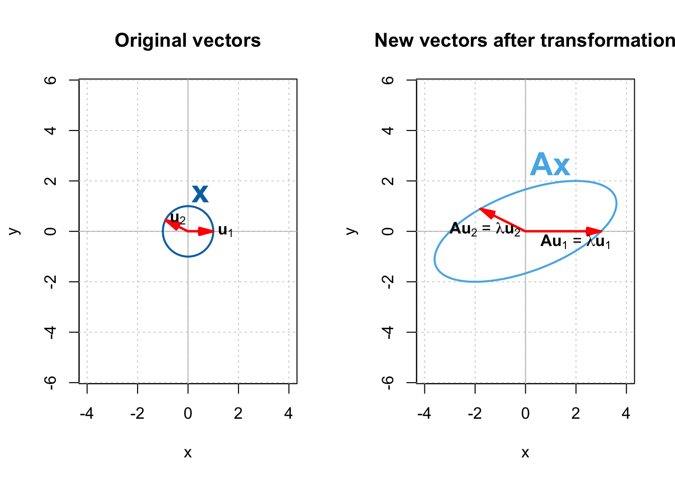
Every vector in $\mathbb{X}$ (left), once transformed by $\mathbf{A}$, is stretched and rotated in $\mathbf{A}\mathbf{x}$ (Figure 1 right), except two vectors — ${\mathbf{u}}_1$ and ${\mathbf{u}}_2$; those are only stretched, as though they are multiplied by a scalar. This is because they are the eigenvectors of $\mathbf{A}$, and multiplying a matrix with its eigenvector is equivalent to multiplying the eigenvector with its corresponding eigenvalue.

$$\mathbf{A}\mathbf{u}=\lambda \mathbf{u}$$

Let’s try another matrix:

$$\mathbf{B}=\left[\begin{array}{cc}3& 1\\ 1& 2\end{array}\right]$$

It’s two eigenvectors:

$${\mathbf{u}}_1=\left[\begin{array}{c}0.8507\\ 0.5257\end{array}\right],{\mathbf{u}}_2=\left[\begin{array}{c}-0.5257\\ 0.8507\end{array}\right]$$

and the corresponding eigenvalues are:

$${\lambda }_1=3.618,{\lambda }_2=1.382$$

Figure 2 shows $\mathbb{X}$ and the eigenvectors of $\mathbf{B}$ — ${\mathbf{u}}_1$ and ${\mathbf{u}}_2$, as well as vectors in $\mathbb{X}$ transformed by $\mathbf{B}$.

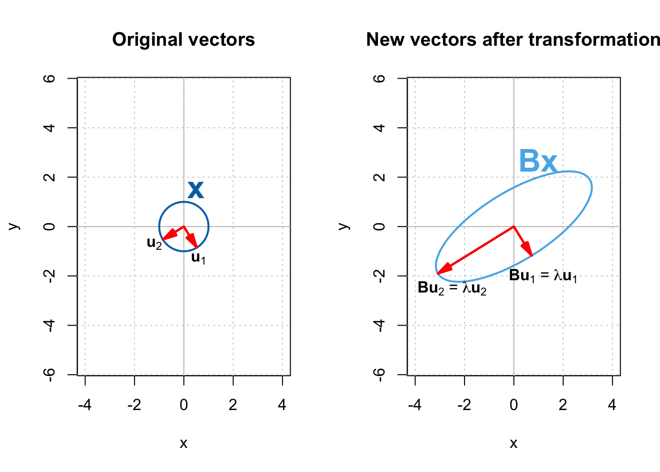
This time, the eigenvectors have an interesting property. They are along the major and minor axes of the ellipse (principal axes), and are perpendicular to each other. An ellipse can be thought of as a circle stretched or shrunk along its principal axes as shown in Figure 2, and matrix $\mathbf{B}$ transforms the initial circle $\mathbb{X}$ by stretching it along ${\mathbf{u}}_1$ and ${\mathbf{u}}_2$, the eigenvectors of $\mathbf{B}$.

How come the eigenvectors of $\mathbf{A}$ did not have this property? This is because $\mathbf{B}$ is a symmetric matrix. A symmetric matrix is a matrix that is equal to its transpose. Here is an example of a symmetric matrix:

$$\left[\begin{array}{cccc}5& 0& 4& 3\\ 0& 7& 9& 2\\ 4& 9& 6& 1\\ 3& 2& 1& 3\end{array}\right]$$

Elements on the main diagonal of a symmetric matrix are arbitrary, but for the other elements, each element on row $i$ and column $j$ is equal to the element on row $j$ and column $i$ ($a_{\text{ij}}=a_{\text{ji}}$). A symmetric matrix is always a square matrix ($n\times n$). Clearly, $\mathbf{A}$ was not symmetric. A symmetric matrix transforms a vector by stretching or shrinking the vector along the eigenvectors of this matrix. In particular, a matrix transforms its eigenvector by multiplying its length (or magnitude) by the corresponding eigenvalue.

Given that the initial vectors in $\mathbb{X}$ all have a length of 1 and that both ${\mathbf{u}}_1$ and ${\mathbf{u}}_2$ are normalized, they are members of $\mathbb{X}$. Their transformed vectors are:

$$\begin{gathered} \mathbf{B}{\mathbf{u}}_1={\lambda }_1{\mathbf{u}}_1, \\ \mathbf{B}{\mathbf{u}}_2={\lambda }_2{\mathbf{u}}_2, \end{gathered}$$

Therefore, the amount of stretching or shrinking along each eigenvector is proportional to the corresponding eigenvalue as shown in Figure 2.

When you have more stretching in the direction of an eigenvector, the eigenvalue corresponding to that eigenvector will be greater. In fact, if the absolute value of an eigenvector is greater than 1, the circle 𝕏 stretches along it; vice versa.

Let’s try another matrix:

$$C=\left[\begin{array}{cc}3& 1\\ 1& 0.8\end{array}\right]$$

The eigenvectors and corresponding eigenvalues are:

$$\begin{gathered} {\mathbf{u}}_1=\left[\begin{array}{c}0.9327\\ 0.3606\end{array}\right], \\ {\mathbf{u}}_2=\left[\begin{array}{c}-0.3606\\ 0.9327\end{array}\right] \end{gathered}$$

$$\begin{array}{r}{\lambda }_1=3.3866,\\ {\lambda }_2=0.4134\end{array}$$

Now if we plot the transformed vectors, we get:

Now we have stretched $\mathbf{x}$ along ${\mathbf{u}}_1$ and shrunk along ${\mathbf{u}}_2$.

In the next post, we will continue discussing eigenvectors, but in the context of a basis for a vector space.