Singular Value Decomposition - Basis

Basis ¶

In Euclidean space $\mathbb{R}^2$, the vectors:

$$ \mathbf{v}_1 = \begin{bmatrix} 1 \\ 0 \\ \end{bmatrix},~ \mathbf{v}_2 = \begin{bmatrix} 0 \\ 1 \\ \end{bmatrix} $$

is the simplest example of a basis. They are linearly independent. They also span $\mathbb{R}^2$ as every vector in $\mathbb{R}^2$ can be expressed as a linear combination of $\mathbf{v}_1$ and $\mathbf{v}_2$. They are called the standard basis for $\mathbb{R}^2$. As a result, the dimension of $\mathbb{R}^2$ is 2.

In general, a set of vectors $\left<\mathbf{v}_1, \mathbf{v}_2, \ldots, \mathbf{v}_n \right>$ form a basis for a vector space $\mathbb{V}$, if they are linearly independent and span $\mathbb{V}$. A vector space is a set of vectors that can be added together or multiplied by scalars. This is a closed set, so when the vectors are added or multiplied by a scalar, the result still belongs to the set. The operations of vector addition and scalar multiplication must satisfy certain requirements which will not be discussed here. Euclidean space $\mathbb{R}^2$ is an example of a vector space.

When a set of vectors is linearly independent, it means that no vector in the set can be written as a linear combination of the other vectors. Therefore, it is not possible to write

$$ \begin{equation*} \mathbf{v}_i = a_1\mathbf{v}_1 + a_2\mathbf{v}_2 + \cdots + a_{i-1}\mathbf{v}_{i-1} + a_{i+1}\mathbf{v}_{i+1} + \cdots + a_n\mathbf{v}_n \end{equation*} $$

when some of $a_1$, $a_2$, $\cdots$, $a_n$ are not zero. In other words, none of the $\mathbf{v}_i$ vectors in this set can be expressed in terms of the other vectors. A set of vectors spans a space if every other vector in the space can be written as a linear combination of the spanning set. Every vector $\mathbf{s}$ in $\mathbb{V}$ can be written as:

$$ \mathbf{s} = a_1\mathbf{v}_1 + a_2\mathbf{v}_2 + \cdots + a_n\mathbf{v}_n $$

A vector space $\mathbb{V}$ can have many different vector bases, but each basis always has the same number of basis vectors. The number of basis vectors of vector space $\mathbb{V}$ is called the dimension of $\mathbb{V}$.

Euclidean space $\mathbb{R}^2$ has other bases other than $\left<\mathbf{v}_1,~\mathbf{v}_2\right>$, but all of them have two vectors that are linearly independent which span $\mathbb{R}^2$.

For example, vectors:

$$ \mathbf{v}_1 = \begin{bmatrix} 1 \\ 1 \\ \end{bmatrix},~ \mathbf{v}_2 = \begin{bmatrix} -1 \\ 1 \\ \end{bmatrix} $$

can also form a basis for $\mathbb{R}^2$.

An important reason to find a basis for a vector space is to form a coordinate system on the basis. If the set of vectors $~B = \left<\mathbf{v}_1, \mathbf{v}_2, \ldots, \mathbf{v}_n \right>~$ form a basis for a vector space, then every vector $\mathbf{x}$ in the space can be uniquely specified using those basis vectors:

$$ \mathbf{x} = a_1\mathbf{v}_1 + a_2\mathbf{v}_2 + \cdots + a_n\mathbf{v}_n $$

Now the coordinate of $\mathbf{x}$ relative to this basis $\mathbb{B}$ is:

$$ \left[\mathbf{x}\right]_B = \begin{bmatrix} a_1 \\ a_2 \\ \vdots \\ a_n \\ \end{bmatrix} $$

In fact, when we are writing a vector in $\mathbb{R}^2$, we are already expressing its coordinate relative to the standard basis. That is because any vector

$$ \mathbf{x} = \begin{bmatrix} a \\ b \\ \end{bmatrix} $$

can be written as

$$ \mathbf{x} = a \begin{bmatrix} 1 \\ 0 \\ \end{bmatrix} + b \begin{bmatrix} 0 \\ 1 \\ \end{bmatrix} $$

In another word, a vector $\mathbf{x}$ is also the coordinate relative to the standard basis of $\mathbb{R}^2$.

Consider: if we know the coordinate of a vector relative to the standard basis, how can we find its coordinate relative to a new (non-standard) basis?

The equation:

$$ \mathbf{x} = a_1\mathbf{v}_1 + a_2\mathbf{v}_2 + \cdots + a_n\mathbf{v}_n $$

can also be written as:

$$ \mathbf{x} = \begin{bmatrix} \mathbf{v}_1 & \mathbf{v}_2 & \cdots & \mathbf{v}_n \\ \end{bmatrix} \begin{bmatrix} a_1 \\ a_2 \\ \vdots \\ a_n \\ \end{bmatrix} = \begin{bmatrix} \mathbf{v}_1 & \mathbf{v}_2 & \cdots & \mathbf{v}_n \\ \end{bmatrix} \left[\mathbf{x}\right]_B = \mathbf{P}_B\left[\mathbf{x}\right]_B $$

The matrix:

$$ \mathbf{P}_B = \begin{bmatrix} \mathbf{v}_1 & \mathbf{v}_2 & \cdots & \mathbf{v}_n \\ \end{bmatrix} $$

is called the change-of-coordinate matrix. The columns of this matrix are the vectors in basis B. The equation

$$ \mathbf{x} = \mathbf{P}_B\left[\mathbf{x}\right]_B $$

gives the coordinate of $\mathbf{x}$ in $\mathbb{R}^2$ (which is simply $\mathbf{x}$ itself) if we know its coordinate in basis B. Likewise, if we need the opposite, we can multiply both sides of this equation by the inverse of the change-of-coordinate matrix to get:

$$ \left[\mathbf{x}\right]_B = \mathbf{P}_B^{-1}\mathbf{x} $$

If we know the coordinate of \mathbf{x} in $\mathbb{R}^2$ (which is simply $\mathbf{x}$ itself), we can multiply it by the inverse of the change-of-coordinate matrix to get its coordinate relative to basis B. For example, suppose that our basis set B is formed by the vectors:

$$ \mathbf{v}_1 = \begin{bmatrix} 1 \\ 0 \\ \end{bmatrix},~ \mathbf{v}_2 = \begin{bmatrix} -1\mathbin{/}\sqrt{2} \\ 1\mathbin{/}\sqrt{2} \\ \end{bmatrix} $$

and we have a vector:

$$ \mathbf{x} = \begin{bmatrix} 2 \\ 2 \\ \end{bmatrix} $$

To calculate the coordinate of $\mathbf{x}$ in B, we form the change-of-coordinate matrix first:

$$ \mathbf{P}_B = \begin{bmatrix} 1 & -1\mathbin{/}\sqrt{2} \\ 0 & 1\mathbin{/}\sqrt{2} \\ \end{bmatrix} $$

Now the coordinate of $\mathbf{x}$ relative to B is:

$$ \left[\mathbf{x}\right]_B = \mathbf{P}_B^{-1}\mathbf{x} = \begin{bmatrix} 1 & -1\mathbin{/}\sqrt{2} \\ 0 & 1\mathbin{/}\sqrt{2} \\ \end{bmatrix}^{-1} \begin{bmatrix} 2 \\ 2 \\ \end{bmatrix} $$

Let’s see how to calculate cooridnates in R. To calculate the inverse of a matrix, we can use function solve().

v_1 <- c(1, 0)
v_2 <- c(-1/sqrt(2), 1/sqrt(2))

# change of coordinate matrix
p_b <- cbind(v_1, v_2)
p_b_inv = solve(p_b)

# cooridnate of x in R^2
x = c(2, 2)

# new coordinate of x relative to basis B
x_coord_b <- p_b_inv %*% x
x_coord_b

        [,1]
v_1 4.000000
v_2 2.828427

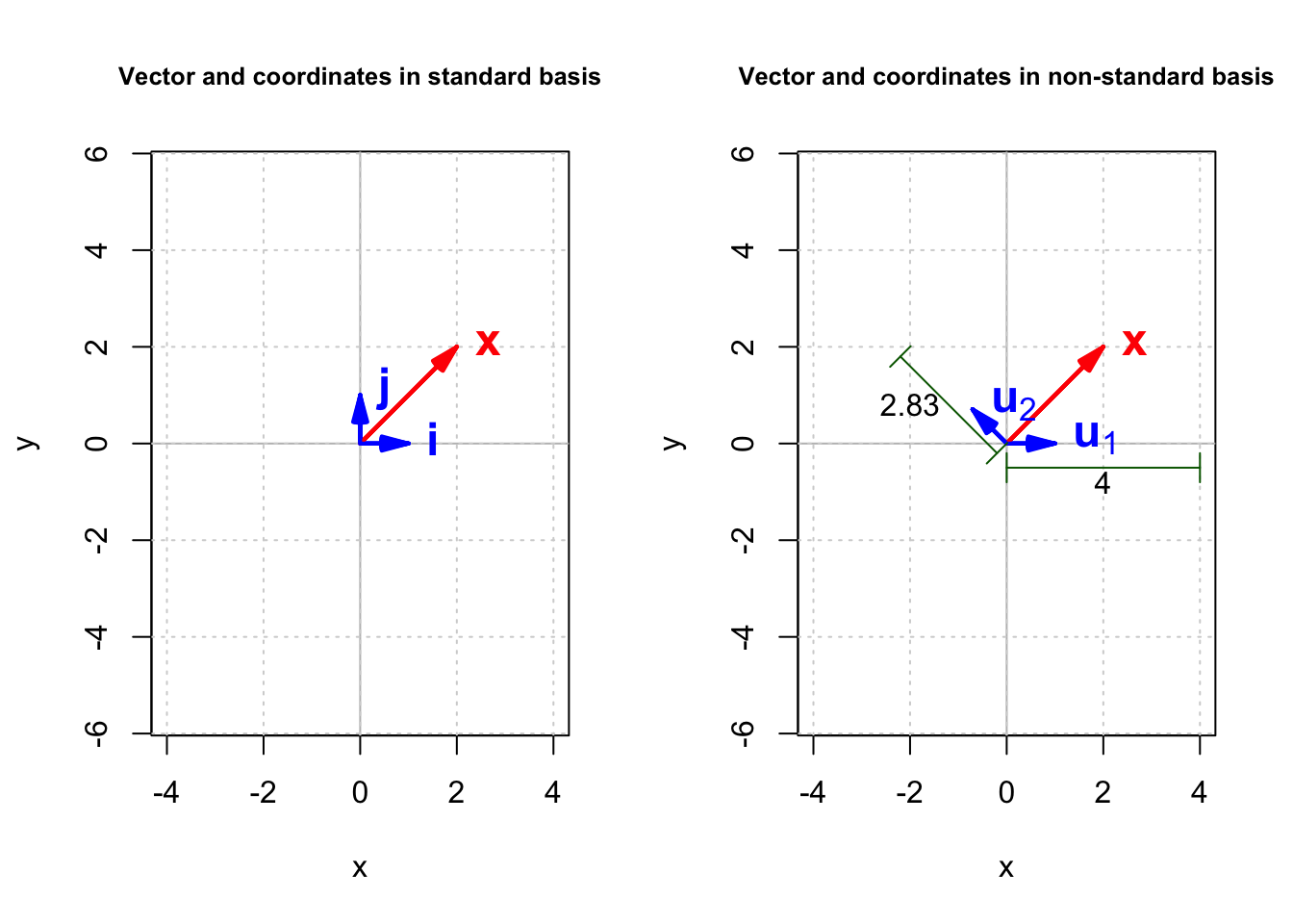
The output show that the coordinate of $\mathbf{x}$ in B is:

$$ \left[\mathbf{x}\right]_B = \begin{bmatrix} 4 \\ 2.8284 \\ \end{bmatrix} $$

Figure 1 shows the effect of changing the basis: $\mathbf{x}$’s coordinates changed from $\left(2,~2 \right)$ to $\left(4,~2.83 \right)$. In general, to find the coordinates of $\mathbf{x}$ in a basis $B$, we can draw a line from the tip of $\mathbf{x}$ parallel to $\mathbf{u}_1$ to find where it intersects with $\mathbf{u}_2$ and another line parallel to $\mathbf{u}_2$ to find where it intersects with $\mathbf{u}_1$. In an $n$-dimensional space, to find the coordinate of $\mathbf{u}_i$, we need to draw a hyper-plane parallel to all other eigenvectors except $\mathbf{u}_i$ which passes the tip of $\mathbf{x}$. Where it intersects $\mathbf{u}_i$ is the coordinate of $\mathbf{x}$ on $\mathbf{u}_i$. This procedure is greatly simplified when eigenvectors are orthogonal. We only need to draw a line from the tip of $\mathbf{x}$ which is perpendicular to the target eigenvector.

If you recall, having orthogonal eigenvectors is an attribute of symmetric matrices. In the next post, we will discuss additional “merits” of symmetric matrices.