Singular Value Decomposition - Intro

Among all the math subjects I have studied during undergraduate — calculus, real analysis, differential equation, probability theory, numerical analysis — matrix algebra was perhaps the least intuitive to me. Many years have gone by, and I have made several attempts since then to re-learn matrix algebra. Until this summer, each past attempt had ended inconspicuously, either because I lost motivation, or because the book I was following along introduced some external dependency and side-tracked me into other rabbit holes with no return tickets. The pattern repeats itself and yet I kept trying. My stubborness is partly because I use statistics heavily in my daily research and work, and matrix algebra is almost around every corner, constantly provoking my curiousity.

Fast forward to this summer. I finally had some free time to indulge in some long-overdue self-development. Once more, I picked up a book on matrix algebra. Halfway through the book, it mentioned in passing “singular value decomposition”. I had never seen this concept before and decided to look it up. By some stroke of luck, I came across a blog post that made matrix algebra “stick” for me. It unpacked the concept so well that many fragmented pieces in matrix algebra I learned in the past started to form a coherent picture in my head. Most important of all, not only is singular value decomposition a beautiful theory, it is also a useful technique and has been applied to compressing images and predicting user preference, among others.

The original blog post walked readers through a series of illustrations rendered in python. Here, I will use R to re-create all the illustrations, with some editorial changes to the original text. You can find the original article by Reza Bagheri here.

Introduction ¶

To understand singular value decomposition, we need to first understand the Eigenvalue Decomposition of a matrix. We can think of a matrix $A$ as a transformation that acts on a vector $x$ by multiplication to produce a new vector $Ax$.

For example, the rotation matrix $\mathbf{A}$ in a 2-$d$ space can be defined as:

$$ \mathbf{A} = \begin{bmatrix} \cos(\theta) & -\sin(\theta) \\ \sin(\theta) & \cos(\theta) \\ \end{bmatrix} $$

This matrix would rotate a vector about the origin by $\theta$.

Another example is the stretching matrix $\mathbf{B}$ in a 2-$d$ space:

$$ \mathbf{B} = \begin{bmatrix} k & 0 \\ 0 & 1 \\ \end{bmatrix} $$ This matrix stretches a vector along the $x$-axis by a constant factor $k$ but does not affect it in the $y$-direction. Similarly, we can have a stretching matrix in $y$-direction.

$$ \mathbf{C} = \begin{bmatrix} 1 & 0 \\ 0 & k \\ \end{bmatrix} $$ As an example, if we have a vector

$$ \mathbf{x} = \begin{bmatrix} 1 \\ 0 \\ \end{bmatrix} $$

then $\mathbf{A}\mathbf{x}$ is the resulting vector after rotating $\mathbf{x}$ by $\theta$, and $\mathbf{B}\mathbf{x}$ is the resulting vector after stretching $\mathbf{x}$ in the $x$-direction by a constant factor $k$.

vec <- c(1, 0) # original vector
theta <- 30 * pi / 180 # 30 degrees in radian
# rotation matrix for theta
mat_rotate <- matrix(c(cos(theta), sin(theta), -sin(theta), cos(theta)), 2)
# stretching matrix for k = 2
mat_stretch <- matrix(c(2, 0, 0, 1), 2)
# vec_rotate is the rotated vector
vec_rotate <- as.vector(mat_rotate %*% vec)
# vec_stretch is the stretched vector
vec_stretch <- as.vector(mat_stretch %*% vec)

# prepare the drawing canvas
# split the canvas into left and right, 1 row by 2 columns,
# with different widths
oldpar <- par(pin = c(1.5, 1))
layout(
  mat = matrix(c(1, 2),
    nrow = 1,
    ncol = 2
  ),
  heights = 1,
  widths = c(1, 1.5)
)
# define the dimensions of canvas
xlim <- c(-0.5, 1.5)
ylim <- c(-0.5, 1)
# plot original and rotated vectors
# axis labels and plot title
plot(
  xlim, ylim, type = "n", xlab = "", ylab = "", main = "Rotation transform", asp = 1
)
# add a reference line to plot and grids
abline(v = 0, h = 0, col = "gray")
grid()
# add vectors to plot
matlib::vectors(
  rbind(vec, vec_rotate),
  col = c("blue", "darkgreen"),
  lwd = c(2, 2),
  angle = 15,
  labels = c(expression(bold(x)), expression(paste(bold(A), bold(x))))
)

# plot original and stretched vectors
# redefine the x-dimension of canvas
xlim <- c(-0.5, 3)
plot(xlim, ylim, type = "n", xlab = "", ylab = "", main = "Stretching transform", asp = 1)
abline(v = 0, h = 0, col = "gray")
grid()
matlib::vectors(
  rbind(vec, vec_stretch),
  col = c("blue", "darkgreen"),
  lwd = c(2, 2),
  angle = 15,
  labels = c(expression(bold(x)), expression(paste(bold(B), bold(x))))
)
par(oldpar)

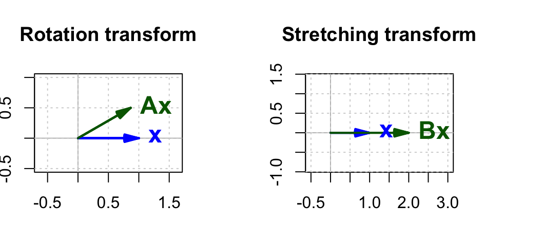
In Figure 1 the rotation matrix is calculated for $\theta = 30^{\circ}$ and the stretching matrix for $k = 2$.

Now we are going to try a different transformation matrix. Suppose that

$$ \mathbf{A} = \begin{bmatrix} 3 & 2 \\ 0 & 2 \\ \end{bmatrix} $$

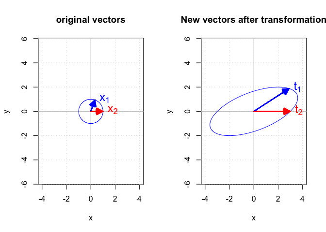
Instead of applying this matrix to a single vector, we apply it to a set of vectors $\mathbb{X}$ that meet the general form of

$$ \mathbf{x} = \begin{bmatrix} x_i \\ y_i \\ \end{bmatrix} \text{where } x_i^2 + y_i^2 = 1 $$

It is easy to see that these vectors are one unit away from the origin $(0, 0)$. Now let’s calculate $\mathbf{t} = \mathbf{A}\mathbf{x}$. $\mathbb{T}$ will be the set of vectors based on $\mathbb{X}$ after being transformed by $\mathbf{A}$.

Figure 2 shows the set of $\mathbb{X}$ and $\mathbb{T}$ and the effect of transforming two sample vectors $\mathbf{x}_1$ and $\mathbf{x}_2$ in $\mathbb{X}$.

 1
 2
 3
 4
 5
 6
 7
 8
 9
10
11
12
13
14
15
16
17
18
19
20
21
22
23
24
25
26
27
28
29
30
31
32
33
34
35
36
37
38
39
40
41
42
43
44
45
46
47
48
49
50
51
52
53
54
55
56
57
58
59
60
61

xi_pos <- seq(from = -1, to = 1, by = 0.01) # top half circle
xi_neg <- seq(from = 1, to = -1, by = -0.01) # bottom half circle
vec_stack <- rbind(
  cbind(
    xi_pos,
    yi = sqrt(1 - xi_pos**2)
  ),
  cbind(
    xi_neg,
    yi = -sqrt(1 - xi_neg**2)
  )
)

x_sample1 <- vec_stack[135, ] # vector x1
x_sample2 <- vec_stack[201, ] # vector x2

# prepare the canvas
# evenly split the canvas into left and right
oldpar <- par(mfrow = c(1, 2))

xlim <- c(-4, 4)
ylim <- c(-4, 4)
plot(xlim, ylim, type = "n", xlab = "x", ylab = "y", main = "original vectors", asp = 1)
abline(v = 0, h = 0, col = "gray")
grid()
# draw the circle
lines(x = vec_stack[, 1], y = vec_stack[, 2], col = "blue")
# draw two vectors x1 and x2
matlib::vectors(
  rbind(x_sample1, x_sample2),
  col = c("blue", "red"),
  lwd = c(2, 2),
  angle = 30,
  labels = c(expression(x[1]), expression(x[2]))
)

# transformation matrix
mat_trans <- matrix(c(3, 0, 2, 2), 2)

# multiply mat_trans with each vector from vec_stack,
# effectively transforming the circule represented by vec_stack
# Not a transparent solution, to optimize [TODO]
vec_stack_trans <- t(apply(vec_stack, MARGIN = 1, FUN = `%*%`, t(mat_trans)))

t_sample1 <- vec_stack_trans[135, ] # vector t1
t_sample2 <- vec_stack_trans[201, ] # vector t2

plot(xlim, ylim, type = "n", xlab = "x", ylab = "y", main = "New vectors after transformation", asp = 1)
abline(v = 0, h = 0, col = "gray")
grid()
lines(x = vec_stack_trans[, 1], y = vec_stack_trans[, 2], col = "blue")
matlib::vectors(
  rbind(t_sample1, t_sample2),
  col = c("blue", "red"),
  lwd = c(2, 2),
  angle = 30,
  labels = c(expression(t[1]), expression(t[2]))
)

# restore default parameter of canvas
par(oldpar)

A word about line 43 in the previous chunk where each vector on the circle was transformed:

43

vec_stack_trans <- t(apply(vec_stack, MARGIN = 1, FUN = `%*%`, t(mat_trans)))

Ideally, I should translate $\mathbf{t} = \mathbf{A}\mathbf{x}$ directly to R code. However, $\mathbb{X}$ was constructed such that each row was a vector $\mathbf{x}$. In another word, each row of $\mathbb{X}$ is $\mathbf{x}^T$. Given that $({\mathbf{A}\mathbf{x}})^T = \mathbf{x}^T\mathbf{A}^T$, therefore $\mathbf{A}\mathbf{x} = ({\mathbf{x}^T\mathbf{A}^T})^T$.

The initial vectors in $\mathbb{X}$ on the left side form a circle, but the transformation matrix $$ \begin{bmatrix} 3 & 2 \\ 0 & 2 \\ \end{bmatrix} $$ turned it into an ellipse.

The sample vectors $\mathbf{x}_1$ and $\mathbf{x}_2$ in the circle are transformed into $\mathbf{t}_1$ and $\mathbf{t}_2$ respectively. So: $$ \begin{align} \mathbf{t}_1 = \mathbf{A}\mathbf{x}_1 \\ \mathbf{t}_2 = \mathbf{A}\mathbf{x}_2 \end{align} $$

In the next post, I will continue this series with eigenvalues and eigenvectors.