Singular Value Decomposition - Rank

Recall that the basis of a vector space $\mathbb{V}$, $⟨{\mathbf{v}}_1,{\mathbf{v}}_2,\dots ,{\mathbf{v}}_n⟩$, are linearly independent and span $\mathbb{V}$. The number of basis vectors for vector space $\mathbb{V}$ is the dimension of $\mathbb{V}$.

A specific type of vector space, column space of matrix $\mathbf{A}$, is written as $\mathrm{col}(\mathbf{A})$. It is defined as the set of all linear combinations of the columns of $\mathbf{A}$, also written as $\mathbf{A}\mathbf{x}$.

Let $\mathbf{A}$ be an $m\times n$ matrix, with column vectors ${\mathbf{v}}_1$, ${\mathbf{v}}_2$, $\dots$, ${\mathbf{v}}_n$.

$$\mathbf{A}=\left[\begin{array}{cccc}{\mathbf{v}}_1& {\mathbf{v}}_2& \cdots & {\mathbf{v}}_n\end{array}\right]$$

A linear combination of theses vectors is therefore

$$c_1{\mathbf{v}}_1+c_2{\mathbf{v}}_2+\cdots +c_n{\mathbf{v}}_n,$$

where $c_1,c_2,\cdots ,c_n$ are scalars. That is, the columns space of $\mathbf{A}$ $\mathrm{col}(\mathbf{A})$ is the span of the vectors ${\mathbf{v}}_1$, ${\mathbf{v}}_2$, $\dots$, ${\mathbf{v}}_n$.

We also have

$$c_1{\mathbf{v}}_1+c_2{\mathbf{v}}_2+\cdots +c_n{\mathbf{v}}_n=\left[\begin{array}{cccc}{\mathbf{v}}_1& {\mathbf{v}}_2& \cdots & {\mathbf{v}}_n\end{array}\right]\left[\begin{array}{c}{c}_1\\ c_2\\ ⋮\\ c_n\end{array}\right]=\mathbf{A}\mathbf{x},$$

where $\mathbf{x}$ is an $n\times 1$ vector, $$\left[\begin{array}{cccc}{c}_1& c_2& \dots & c_n\end{array}\right].$$

Therefore, column space $\mathrm{col}(\mathbf{A})$ consists of all vectors in the form of $\mathbf{A}\mathbf{x}$. Like any other vector space, a column space also has basis vectors. The number of basis vectors for $\mathrm{col}(\mathbf{A})$, or the dimension of $\mathrm{col}(\mathbf{A})$ is called the rank of $\mathbf{A}$. In other words, the rank of $\mathbf{A}$ is the dimension of column space $\mathbf{A}\mathbf{x}$.

The rank of $\mathbf{A}$ is also the maximum number of linearly independent columns in $\mathbf{A}$. This is because we can write all the dependent columns as a linear combination of these linearly independent columns. Given that $\mathbf{A}\mathbf{x}$ consists of all possible linear combination of columns in $\mathbf{A}$, any member in $\mathbf{A}\mathbf{x}$ can also be written as a linear combination of these linearly independent columns. These linearly independent columns span $\mathbf{A}\mathbf{x}$ and form a basis for $\mathrm{col}(\mathbf{A})$, and the number of these vectors becomes the dimension of $\mathrm{col}(\mathbf{A})$ or rank of $\mathbf{A}$.

In the previous post on eigendecomposition, the rank of each projection matrix ${\lambda }_i{\mathbf{u}}_i{\mathbf{u}}_i^T$ is 1. Recall that each projection matrix only have one non-zero eigenvalue. This is not a coincidence. It can be shown that the rank of a symmetric matrix is equal to the number of its non-zero eigenvalues.

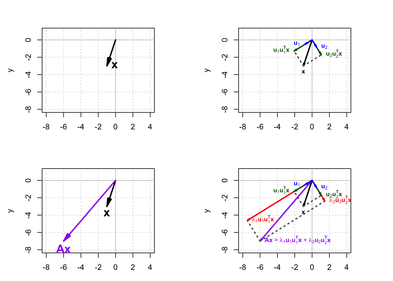
Let’s return to the eigendecomposition equation. Suppose that we apply our symmetric matrix $\mathbf{A}$ to an arbitrary vector $\mathbf{x}$. Now the eigendecomposition equation becomes:

$$\mathbf{A}\mathbf{x}={\lambda }_1{\mathbf{u}}_1{\mathbf{u}}_1^{\mathrm{\top }}\mathbf{x}+{\lambda }_2{\mathbf{u}}_2{\mathbf{u}}_2^{\mathrm{\top }}\mathbf{x}+\cdots +{\lambda }_n{\mathbf{u}}_n{\mathbf{u}}_n^{\mathrm{\top }}\mathbf{x}$$

Recall the important property of symmetrix matrices in the last post. An $n\times n$ symmetric matrix has $n$ real eigenvalues, as well as $n$ linear independent and orthogonal eigenvectors. These eigenvectors can be used as a new basis of a $n\times 1$ vector $\mathbf{x}$. In other words, a $n\times 1$ vector $\mathbf{x}$ can be uniquely written as a linear combination of the eigenvectors of $\mathbf{A}$

$$\mathbf{x}=a_1{\mathbf{u}}_1+a_2{\mathbf{u}}_2+\cdots +a_n{\mathbf{u}}_n,$$

$${\left[x\right]}_B=\left[\begin{array}{c}{a}_1\\ a_2\\ ⋮\\ a_n\end{array}\right]$$

Recall that all the eigenvectors of a symmetric matrix are orthogonal. To find each coordinate $a_i$, we just need to draw a line perpendicular to an axis of ${\mathbf{u}}_i$ through point $\mathbf{x}$ and see where they intersect. Therefore, each coordinate $a_i$ is equal to the dot product of $\mathbf{x}$ and ${\mathbf{u}}_i$, and $\mathbf{x}$ can be re-written as

$$\mathbf{x}=({\mathbf{u}}_1^{\mathrm{\top }}\mathbf{x}){\mathbf{u}}_1+({\mathbf{u}}_2^{\mathrm{\top }}\mathbf{x}){\mathbf{u}}_2+\cdots +({\mathbf{u}}_n^{\mathrm{\top }}\mathbf{x}){\mathbf{u}}_n$$

Now if we multiply $\mathbf{A}$ by $\mathbf{x}$, we get:

$$\mathbf{A}\mathbf{x}=({\mathbf{u}}_1^{\mathrm{\top }}\mathbf{x})\mathbf{A}{\mathbf{u}}_1+({\mathbf{u}}_2^{\mathrm{\top }}\mathbf{x})\mathbf{A}{\mathbf{u}}_2+\cdots +({\mathbf{u}}_n^{\mathrm{\top }}\mathbf{x})\mathbf{A}{\mathbf{u}}_n$$

and since the ${\mathbf{u}}_i$ vectors are eigenvectors of $\mathbf{A}$, the last equation simplies to:

$$\begin{array}{rl}\mathbf{A}\mathbf{x}& =({\mathbf{u}}_1^{\mathrm{\top }}\mathbf{x}){\lambda }_1{\mathbf{u}}_1+({\mathbf{u}}_2^{\mathrm{\top }}\mathbf{x}){\lambda }_2{\mathbf{u}}_2+\cdots +({\mathbf{u}}_n^{\mathrm{\top }}\mathbf{x}){\lambda }_n{\mathbf{u}}_n\\ & ={\lambda }_1{\mathbf{u}}_1{\mathbf{u}}_1^{\mathrm{\top }}\mathbf{x}+{\lambda }_2{\mathbf{u}}_2{\mathbf{u}}_2^{\mathrm{\top }}\mathbf{x}+\cdots +{\lambda }_n{\mathbf{u}}_n{\mathbf{u}}_n^{\mathrm{\top }}\mathbf{x}\end{array}$$

which is the eigendecomposition equation.

Each of the eigenvectors ${\mathbf{u}}_i$ is normalized, so they are unit vectors. In each term of the eigendecomposition equation, ${\mathbf{u}}_i{\mathbf{u}}_i^T\mathbf{x}$ gives a new vector which is the orthogonal projection of $\mathbf{x}$ onto ${\mathbf{u}}_i$. Then this vector is scaled by ${\lambda }_i$. Finally all the $n$ vectors ${\lambda }_i{\mathbf{u}}_i{\mathbf{u}}_i^{\mathrm{\top }}\mathbf{x}$ are summed together to give $\mathbf{A}\mathbf{x}$. This process is shown in Figure 1.

The eigendecomposition mathematically explains an important property of symmetric matrices that we have seen in the plots before. A symmetric matrix transforms a vector by stretching or shrinking it along its eigenvectors, and the amount of stretching or shrinking along each eigenvector is proportional to the corresponding eigenvalue.

In addition, the eigendecomposition can break an $n\times n$ symmetric matrix into $n$ matrices with the same shape ($n\times n$) multiplied by one of the eigenvalues. The eigenvalues play an important role here since they can be thought of as a multiplier. The projection matrix only projects $\mathbf{x}$ onto each ${\mathbf{u}}_i$, and the eigenvalue scales the length of the vector projection (${\mathbf{u}}_i{\mathbf{u}}_i^{\mathrm{\top }}\mathbf{x}$). The bigger the eigenvalue, the bigger the length of the resulting vector (${\lambda }_i{\mathbf{u}}_i{\mathbf{u}}_i^{\mathrm{\top }}\mathbf{x}$) is, and the more weight is given to its corresponding matrix (${\mathbf{u}}_i{\mathbf{u}}_i^{\mathrm{\top }}$).

We can approximate the original symmetric matrix $\mathbf{A}$ by summing the terms which have the highest eigenvalues. For example, if we assume the eigenvalues ${\lambda }_i$ have been sorted in descending order,

$$\mathbf{A}={\lambda }_1{\mathbf{u}}_1{\mathbf{u}}_1^{\mathrm{\top }}+{\lambda }_2{\mathbf{u}}_2{\mathbf{u}}_2^{\mathrm{\top }}+\cdots +{\lambda }_n{\mathbf{u}}_n{\mathbf{u}}_n^{\mathrm{\top }},$$

$${\lambda }_1\ge {\lambda }_2\ge \cdots \ge {\lambda }_n$$

then we can take only the first $k$ terms in the eigendecomposition equation to have a good approximation for the original matrix:

$$\mathbf{A}\approx {\mathbf{A}}_k={\lambda }_1{\mathbf{u}}_1{\mathbf{u}}_1^{\mathrm{\top }}+{\lambda }_2{\mathbf{u}}_2{\mathbf{u}}_2^{\mathrm{\top }}+\cdots +{\lambda }_k{\mathbf{u}}_k{\mathbf{u}}_k^{\mathrm{\top }}$$

where $\mathbf{A}\mathbf{k}$ is an approximation of $\mathbf{A}$ with the first $k$ terms.

If in the original matrix $\mathbf{A}$, the other $(n-k)$ eigenvalues that we left out are very small and close to zero, then the approximated matrix in a very similar to the original matrix, and we have a good approximation.

Matrix

$$\mathbf{C}=\left[\begin{array}{cc}5& 1\\ 1& 0.35\end{array}\right]$$

with

$${\lambda }_1=5.206,{\lambda }_2=0.144$$

$${\mathbf{u}}_1=\left[\begin{array}{c}-0.979\\ -0.202\end{array}\right],{\mathbf{u}}_2=\left[\begin{array}{c}0.202\\ -0.979\end{array}\right]$$

is an example. Here ${\lambda }_2$ is very small compared to ${\lambda }_1$. We could approximate $\mathbf{C}$ with its first term in eigendecomposition corresponding to eigenvalue ${\lambda }_1$. Let’s visualize this by applying $\mathbf{C}$ to vectors on a unit circle.

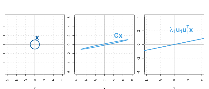
Multiplying $\mathbf{x}$ by $\mathbf{C}$ results in a very similar shape compared to multiplying $\mathbf{x}$ by ${\lambda }_1{\mathbf{u}}_1{\mathbf{u}}_1^{\mathrm{\top }}$.

Keep in mind that a symmetric matrix is required for the eigendecomposition equation to hold. Suppose that you have a non-symmetric matrix:

$$\left[\begin{array}{cc}3& -1\\ 1& 2\end{array}\right]$$

the eigenvectors are not linear independent, and the eigenvalues have both real and imaginary parts. Without real eigenvalues, we cannot properly scale projected vectors.

Or consider another non-symmetric matrix:

$$\left[\begin{array}{cc}3& 2\\ 0& 2\end{array}\right]$$

Here the eigenvectors are linearly independent, but are not orthogonal, and they do not show the correct direction of stretching after transformation.

The eigendecoposition method is very useful, but only works for a symmetric matrix. A symmetric matrix is always a square matrix. If you have a non-square matrix, or a square but non-symmetric matrix, then you cannot use the eigendecomposition method to approximate it with other matrices. Singular Value Decomposition overcomes this problem, which will the topic of our next post.