Singular Value Decomposition - Eigenvalue

In the last post, I described matrix as a transformation mapped onto one or multiple vectors. In this sequel, we continue building the foundation that leads to Singular Value Decomposition.

Eigenvalues and Eigenvectors ¶

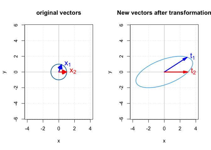
A vector is an entity which has both magnitude and direction. The general effect of matrix $\mathbf{A}$ on a vector in $\mathbb{X}$ is a combination of stretching and rotation. For example, in Figure 1, matrix $\mathbf{A}$ changed both direction and magnitude of vector ${\mathbf{x}}_1$, which resulted in the transformed vector ${\mathbf{t}}_1$. However, for vector ${\mathbf{x}}_2$, only its magnitude changed after transformation. ${\mathbf{x}}_2$ and ${\mathbf{t}}_2$ have the same direction. Matrix $\mathbf{A}$ only stretched ${\mathbf{x}}_2$ in the same direction and returned vector ${\mathbf{t}}_2$ which has a bigger magnitude.

The only way to change the magnitude of a vector without changing its direction is by multiplying it with a scalar. For example, we have a vector $\mathbf{u}$ and a scalar quantity $\lambda$, then $\lambda \mathbf{u}$ has the same direction and a different magnitude as $\mathbf{u}$. For a vector like ${\mathbf{x}}_2$ in Figure 1, the effect of multiplying by $\mathbf{A}$ is like multiplying it with a scalar quantity $\lambda$.

$${\mathbf{t}}_2=\mathbf{A}{\mathbf{x}}_2=\lambda {\mathbf{x}}_2$$

This is not universally true for all vectors in $\mathbb{X}$. In fact, for a given matrix $\mathbf{A}$, only some vectors in $\mathbb{X}$ have this property. These special vectors are called the eigenvectors of matrix $\mathbf{A}$ and their corresponding scalar quantity $\lambda$ is called an eigenvalue of matrix $\mathbf{A}$ for that eigenvector. The eigenvector of an $n\times n$ matrix $\mathbf{A}$ is defined as a nonzero vector $\mathbf{u}$ such that:

$$\mathbf{A}\mathbf{u}=\lambda \mathbf{u}$$

where $\lambda$ is a scalar and is called the eigenvalue of $\mathbf{A}$, and $\mathbf{u}$ is the eigenvector corresponding to $\lambda$. In addition, if you have any other vectors in the form of $a\mathbf{u}$ where $a$ is a scalar, then by placing it in the previous equation we get: $$\mathbf{A}(a\mathbf{u})=a\mathbf{A}\mathbf{u}=a\lambda \mathbf{u}=\lambda (a\mathbf{u})$$

which means that any vector which has the same direction as the eigenvector $\mathbf{u}$ (or the opposite direction if $a$ is negative) is also an eigenvector with the same corresponding eigenvalue. For example, the eigenvalues of $$\mathbf{B}=\left[\begin{array}{cc}-1& 1\\ 0& -2\end{array}\right]$$ are ${\lambda }_1=-1$ and ${\lambda }_2=-2$ and their corresponding eigenvectors are:

$${\mathbf{u}}_1=\left[\begin{array}{c}1\\ 0\end{array}\right]$$

$${\mathbf{u}}_2=\left[\begin{array}{c}-1\\ 1\end{array}\right]$$

and we have:

$$\begin{array}{r}\mathbf{B}{\mathbf{u}}_1={\lambda }_1{\mathbf{u}}_1\\ \mathbf{B}{\mathbf{u}}_2={\lambda }_2{\mathbf{u}}_2\end{array}$$

This means that when we apply matrix $\mathbf{B}$ to all the possible vectors, it does not change the direction of two vectors — ${\mathbf{u}}_1$ and ${\mathbf{u}}_2$ (or any vectors which have the same or opposite direction) — but only stretches them. For eigenvectors, matrix multiplication turns into a simple scalar multiplication.

Next, we calculate eigenvalues and eigenvectors of $\mathbf{B}$ using R.

# target matrix
mat_b <- matrix(c(-1, 0, 1, -2), 2)
# calculate eigenvalues and eigenvectors for `mat_b`
eigen_b <- eigen(mat_b)
eigen_b

eigen() decomposition
$values
[1] -2 -1

$vectors
           [,1] [,2]
[1,] -0.7071068    1
[2,]  0.7071068    0

We used function eigen() from base R to calculate the eigenvalues and eigenvectors. It returned a list. The first element of this list is a vector that stores the eigenvalues. The second element is a matrix that stores the corresponding eigenvectors.

Note that the eigenvector for ${\lambda }_2=-1$ is the same as ${\mathbf{u}}_2$,

$$\left[\begin{array}{c}1\\ 0\end{array}\right]$$

but the eigenvector for ${\lambda }_1=-2$ is different from ${\mathbf{u}}_1$. That is because eigen() returns the normalized eigenvector. A normalized vector is a unit vector whose magnitude is 1. Before explaining how to calculate the magnitude of a vector, we need to learn the transpose of a matrix and the dot product, which will be the topic of my next post.