Module 1 Programming Bootcamp
Programming languages go in and out of style. To be a strong programmer, it is important to understand not just the ins and outs of a particular programming language, but how computer languages and computing infrastructure work more generally. In this course, learners are first introduced to some of the core concepts of computer programming in a language-agnostic way, before being shown the basics of R and Python, two of the most common programming languages used in modern data analysis.
Intended audience
This course is intended as a primer for individuals without programming experience. It is not intended for people with existing programming experience.
Pre-requisites
Exposure to programming framewors would be beneficial but is not necessary.
Learning outcomes
Develop awareness of fundamental concepts that can be applied to any programming language
Gain insight into what is common across all computer languages
Provide steps to learning any programming language, through reference to these common fundamentals
Allow learners to implement the notions taught in the Introduction and Advanced courses in R and/or Python
At the end of this course, participants will have acquired fundamental concepts of programming that apply to all computer languages, preparing them for success in introductory and advance courses using R and Python.
1.1 Programming fundamentals
1.1.1 Code components
1.1.2 Designing with pseudo-code
1.1.3 From pseudo-code to code that runs
1.2 Basics of R
R is a powerful language that is widely-used for data analysis and statistical computing. It was developed in the early 90s by Ross Ihaka and Robert Gentleman. Since then, continuous efforts have been made to improve R’s user interface. The journey of R language from a rudimentary text editor to interactive R Studio and more recently Jupyter Notebooks has engaged many data science communities across the world.
This was made possible in part because of generous contributions by R
users. The inclusion of sophisticated packages (such as dplyr,
tidyr, readr, data.table, SparkR, ggplot2, etc.) has made R
both more powerful and more useful, allowing for smart data
manipulation, visualization, and computation.
1.2.1 Why Use R?
Here are some benefits that potential users might note:
the style of coding is intuitive;
R is open source and free;
more than 7800 packages, customized for various computation tasks, are available (as of October 2017);
the R community is overwhelmingly welcoming and useful to new users and experienced users alike (you can browse and ask questions at StackOverflow, and consult worked-out examples on R-bloggers, for instance);
high performance computing experience is possible (with the appropriate packages), and
is is one of the highly sought skills by analytics and data science companies.
1.2.2 Installing R / R Studio
Note: If you have a pre-existing installation of R and/or RStudio, you may skip this part. However, we highly recommend that you upgrade both to the latest version, if they have not been upgraded for a while. Consult Section 1.6.1 if you are not sure how to upgrade.
You can download and install the vanilla version of R, but the addition of RStudio provides a much better coding experience, in our opinion. The following steps will allow you to install R and R Studio (yes, you would need both).
- You must do this first:
Download and install R by going to https://cloud.r-project.org/.
- If you are a Windows user: Click on Download R for Windows,
then click on base, then click on the Download R X.X.X for Windows link,
where
R X.X.Xis the version number. For example, the latest version of R as of 2021-11-01, wasR 4.1.2. - If you are a macOS user: Click on Download R for macOS,
then under “Latest release::” click on R-X.X.X.pkg,
where
R-X.X.Xis the version number. If your Mac has an Arm-based M1 chip, choose the R-X.X.X-arm64.pkg instead. - If you are a Linux user: Click on Download R for Linux and choose your distribution for more information on installing R for your setup.
- If you are a Windows user: Click on Download R for Windows,
then click on base, then click on the Download R X.X.X for Windows link,
where
- You must do this second:
Download and install RStudio at
https://www.rstudio.com/products/rstudio/download/#download.
- Look for a big blue button that says
DOWNLOAD RSTUDIO FOR …, where
...is your operating system. - Click on the button to start downloading
- Once downloading has completed, double-click it to open, and follow the installation instruction.
- Look for a big blue button that says
DOWNLOAD RSTUDIO FOR …, where
- Complete this additional step only if you are a macOS user:
Download and install XQuartz.
- Go to https://www.xquartz.org. Under “Quick Download”, click on “XQuartz-2.8.1.dmg”.
- Save the
.dmgfile, double-click it to open, and follow the installation instructions (you may need to restart your computer). - Reminder: you will need to re-install XQuartz when upgrading your macOS to a new major version.
- Even though we have installed both R and RStudio,
we will always be working with RStudio from this point on,
knowing that RStudio is nothing but a nice shell over the engine that is
R. Once you open RStudio, the RStudio GUI will display 4 panes (Figure 1.1):
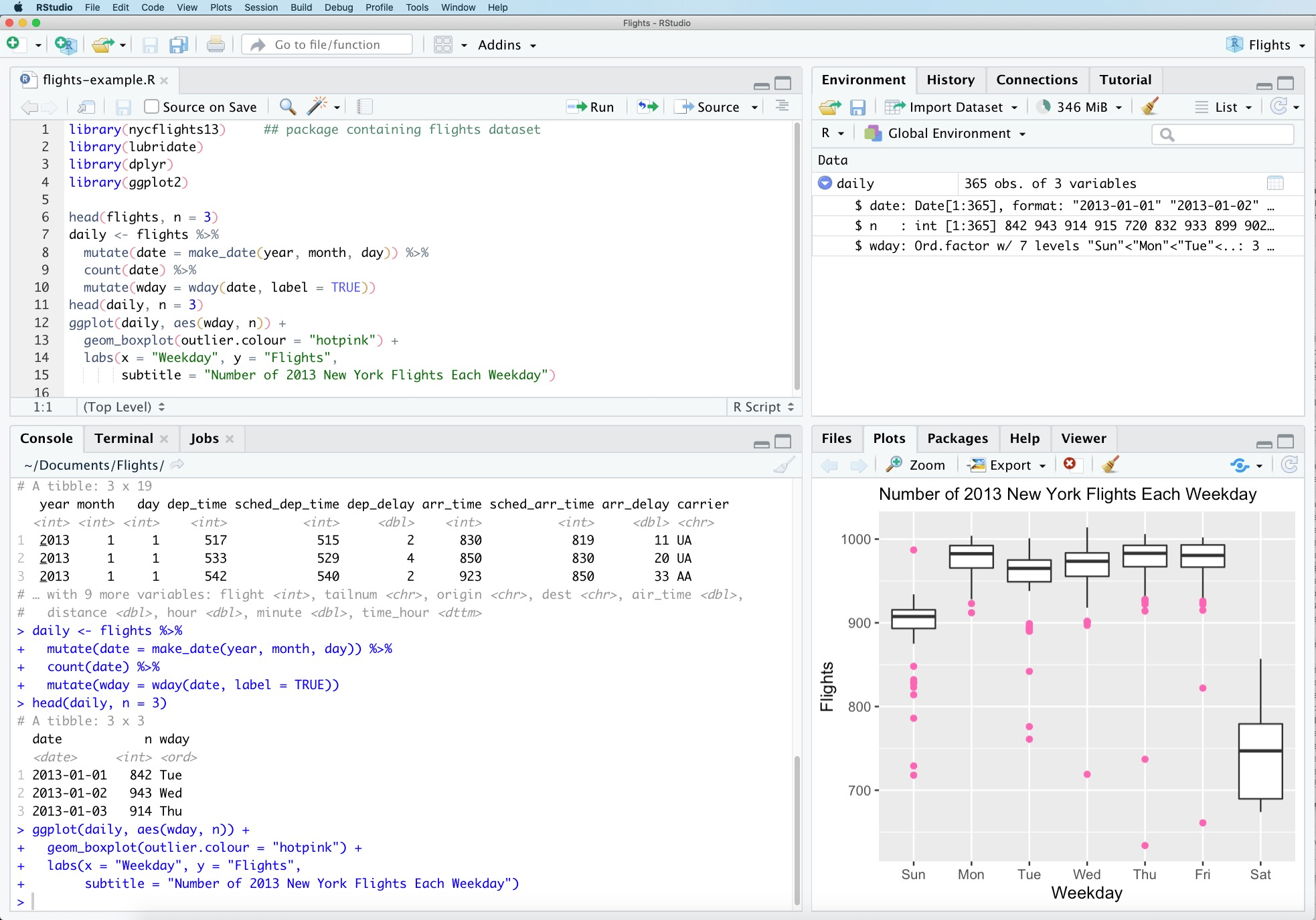
Figure 1.1: RStudio interface.
Console: this area shows the output of code that has been run (either from the command line in the console or from the script window).
Script: as the name suggests, this is the area one would typically use to write code. Lines can be run by first selecting them (right-clicking) and pressing
ctrl + enter(win) orcmd + enter(mac) simultaneously. Alternatively, you can click on the little ‘Run’ button located at the top right corner of the script window.Environment: this space displays the set of external elements that have been added. This includes data set, variables, vectors, functions etc. This area allows the user to verify that data has been loaded properly.
Graphical Output: this space display the graphs created during exploratory data analysis, or embedded help on package functions from R’s official documentation.
1.2.3 Test test test
To make sure you have installed both R and RStudio properly,
type a simple command.
For example, place your cursor in the pane labelled Console,
type x <- 2 + 2, followed by enter or return.
Then type x followed by enter or return.
You should see the value 4 printed to the screen.
If yes, you’ve successfully installed R and RStudio.
1.2.4 Customize your RStudio
Even if you had preivously installed R and RStudio, I encourage you not to skip this part. There might be some recommended setting you have not done despite your familiarity with R and/or RStudio.
In RStudio, go to Tools >> Global Options, make these changes to the setting as described in Figure 1.2:
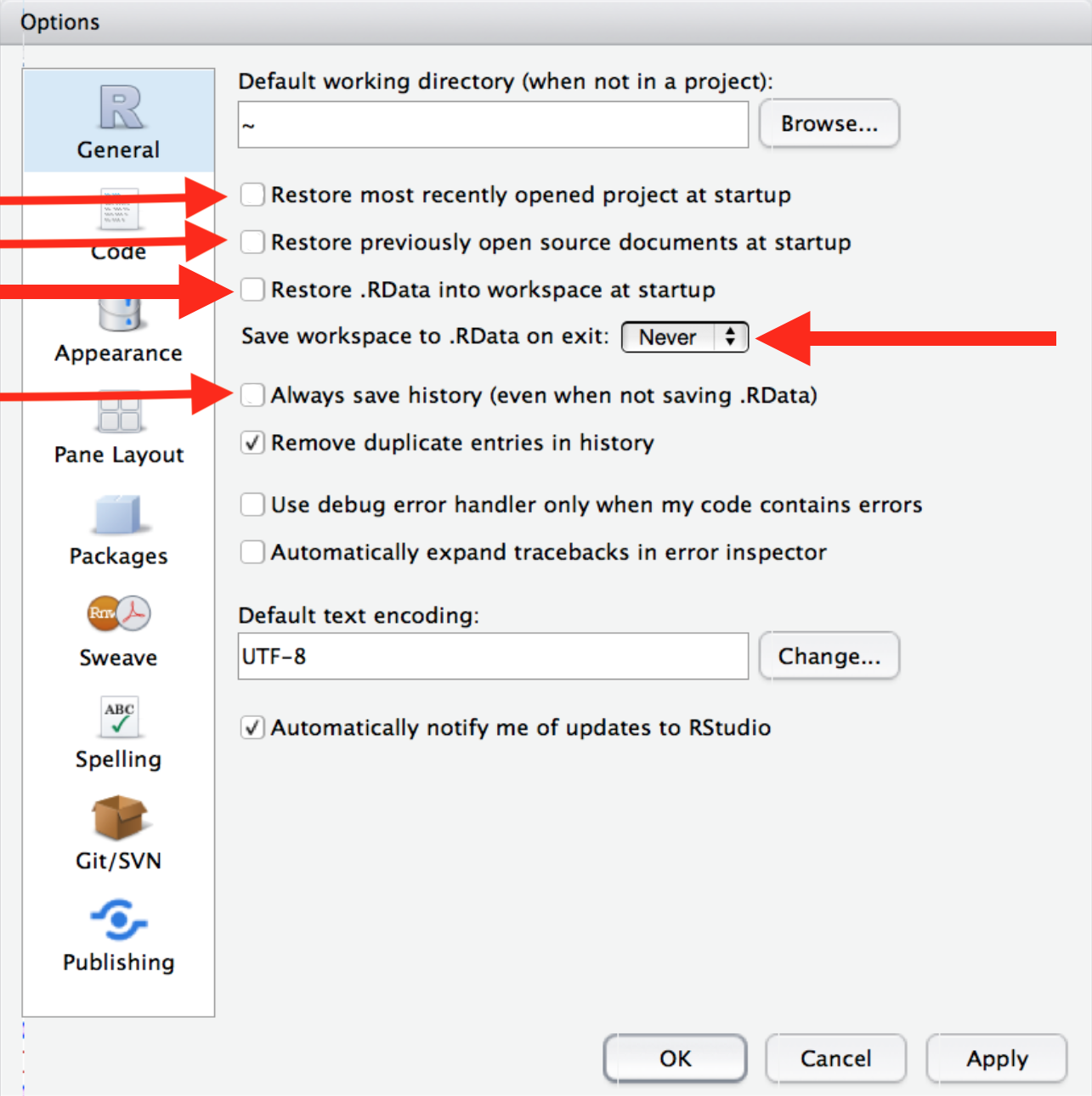
Figure 1.2: Start R with a blank slate, from R for Data Science, chapter 8, with modifications.
[These settings] will cause you some short-term pain, because now when you restart RStudio it will not remember the results of the code that you ran last time. But this short-term pain will save you long-term agony because it forces you to capture all important interactions in your source code. There’s nothing worse than discovering three months after the fact that you’ve only stored the results of an important calculation in your workspace, not the calculation itself in your source code.
Optionally, you could also adjust the font size via Tools >> Global Options >> Appearance >> Editor font size. By default, it is set at 12. I find size 14 easier on my eyes.
1.2.5 Elements of code in base R
1.2.6 tidyverse
1.3 Basics of python
This is a test of cross-reference. As we have discussed in 1.2, you can have different data types.
1.3.1 Elements of code in python
1.3.2 pandas and numpy
1.4 Other programming frameworks
1.5 Short Examples - Programming in R
Many software packages and libraries are available to the data analyst. R not only has the advantage that we can easily use its available packages, but it provides enough flexibility for the analyst who wants to get dirty with the data. It’s also widely used, and thus fairly portable: most analysts speak some level of R (or something that sounds and looks an awful lot like R).
In this notebook, you will find examples and tips that highlight R’s data manipulation features. It is not meant to be a complete introduction, or even a showcase of good programming practices.
1.5.1 Packages and Libraries
While it is possible to write command line functions in R (we’ll have a few in subsequent modules), we will mostly use routines and functions which are available through various packages and libraries.
With an Internet connection, it is fairly straightforward to install and/or update R packages.
1.5.2 Commonly Used Libraries
(to be added to continuously…)
- Outlier Detection: outlier, EVIR
- Feature Selection: Features, RRF
- Data Transformation: plyr, data.table
- Data Visualization: ggplot2, googleVis, graphics, GGally
- Text Mining: tm, wordcloud
- Dimension Reduction: factoMiner, CCP
- Imputation: MissForest, MissMDA
- Association Rules: arules, arulesViz
- Decision Trees: rpart, party, rattle, rpart.plot, randomForest, RGtk2, ctree
- Clustering: stats, cluster, apcluster
- ANNs: nnet, neuralnet
- SVMs: e1071, libsvm, kernlab
- Summary Statistics: psych
- Analysis: stats
- Baseball: lahman
- Other: stringr
1.5.3 Help and Documentation
R’s various help files and demos can be accessed using the following commands (where function_name and search_term correspond to the desired function and/or term):
?function_nameexample(function_name)args(function_name)??search_term
We can copy code from the example file, and run it directly.
counts <- c(18,17,15,20,10,20,25,13,12)
outcome <- gl(3,1,9)
treatment <- gl(3,3)
print(d.AD <- data.frame(treatment, outcome, counts))
glm.D93 <- glm(counts ~ outcome + treatment, family = poisson())
anova(glm.D93)
summary(glm.D93)
The function’s arguments can be accessed via args().
1.5.4 The R Workspace
How do we arrange for data to be made available in the R workspace?
We can either use built-in datasets, or we can load data from external sources.
1.5.4.1 Loading a Built-In Dataset
# uncomment to list datasets in all available packages
# data(package = .packages(all.available = TRUE))
Let’s take a look at three datasets:
- swiss
- volcano
- InsectSprays
1.5.4.2 Loading an External Dataset
Data <- read.csv("path_name/file_name", header=TRUE, sep=",")#CSV fileData <- read.table("path_name/file_name", sep="\t", header=TRUE)#tab separatedData <- read.table(file = "clipboard", sep="\t", header=TRUE)#clipboardData <- read.csv("http://dns/path_name/file")#web
1.5.4.3 Removing and Saving Workplace Objects
rm(variable_x)#removing variable_x from the workspacesave.image()#saving entire workspacesave(variable_name, file=“file_name.rda”)#saving a specific objectload(“file_name.rda”)#saving a specific object
1.5.5 Simple Data Manipulation
So what can we actually do with R?
1.5.5.1 Assigning Data
1.5.5.2 Data Types and Conversion
# test if an object is of a certain type - I
is.numeric(x)
is.character(x)
is.vector(x)
is.matrix(x)
is.data.frame(x)
# set an object as a specific type
as.numeric(x)
as.character(x)
as.vector(x)
as.matrix(x)
as.data.frame(x)1.5.5.3 Writing Function
What if we’re interested in writing our own functions in R?
The template for all functions is a block of code that looks like:
my.function <- function(arg1,arg2, ..., argn) {
# what my.function does, typically involving the arguments
}
Here are some simple examples:
1.5.6 Exploring Data
Let’s take a look at the swiss dataset in detail.
# Display the first few entries of the dataset
head(swiss,8)   # setting a different number of observations, 10 in this case
# Display a specific column as a data frame
swiss$Education # extracting a specific colum with the $ operator
#swiss_matrix$Education # this cannot be done to a matrix
swiss_matrix[,4]# Displaying specific entries, rows, and columns using matrix notation
swiss[1,1] # 1st row, 1st column
swiss[1,] # 1st row
swiss[,2] # 2nd column
swiss[c(2,4),] # 2nd and 4th rows
swiss[,c(2,4)] # 2nd and 4th columns
swiss[,-2] # all rows without the 2nd column
swiss[-3,] # all columns without the 3rd row# column names
colnames(swiss)
# row names
rownames(swiss)
# structure of the data frame
str(swiss)
# summary statistics
summary(swiss) # summary statistics of the data frame (5pt-summary + mean for numeric variables )
library(psych)
describe(swiss) # matrix of data fame statistics: n, mean, sd, median, min, max, range, skew, kurtosis, se, + others
cor(swiss) # correlation matrix of the data# Contrast: dataset with categorical variables
summary(InsectSprays) # count for categorical variables
table(InsectSprays) # joint empirical distribution ... not really useful here
str(InsectSprays)
describe(InsectSprays) # look at the statistics for the categorical variable
# cor(InsectSprays) # uncomment to see what happens if there are categorical variables# finding all observations for which a feature takes on a value greater than a threshold
swiss$Fertility>50# historical provinces for which Fertility was > 50
swiss[swiss$Fertility>50,]
# number of such historical cantons
nrow(swiss[swiss$Fertility>50,]) # should be at most as large as the number of observations# historical provinces data where Fertility is in the top 50%
swiss[swiss$Fertility>median(swiss$Fertility),]
# Fertiliy and Education variables for historical cantons where Fertility is in the top 50%
swiss[swiss$Fertility>median(swiss$Fertility),c(1,4)] # matrix option
swiss[swiss$Fertility>median(swiss$Fertility),c("Fertility","Education")] # data frame call
# historical canton(s) data where Fertility is maximal
swiss[swiss$Fertility == max(swiss$Fertility),]# find the historical cantons for which the first variable is in the top 50%
swiss$var1 <- swiss[,1]>median(swiss[,1])
# find the historical cantons for which the fourth variable is in the top 50%
swiss$var4 <- swiss[,4]>median(swiss[,4])
# distribution of cantons about the median of the first variable
table(swiss$var1)
# distribution of cantons about the median of the fourth variable
table(swiss$var4)
# what’s going on here? rows = first variable, columns = second variable
table(swiss$var1,swiss$var4) 1.5.7 A Word About NAs
NA values in R can create some havoc. Be careful!
# create a dataset
# by picking 100 values (with replacement) among the values {1,2,3,4,NA}
test = sample(c(1:4,NA),100, replace=TRUE)

summary(test)   # 5pt summary + mean + number of NAs

mean(test)   # mean of test data without removal of the NAs
# mean of test data with removal of the NAs
mean(test, na.rm=TRUE)
# median of test data with removal of the NAs
median(test, na.rm=TRUE)
# minimum of test data with removal of the NAs
min(test, na.rm=TRUE)
# maximum of test data with removal of the NAs
max(test, na.rm=TRUE)
# quantiles of test data with removal of the NAs
quantile(test, na.rm=TRUE) 1.6 Additional resources
1.6.1 Upgrade R and/or RStudio
There are many ways to upgrade R and/or RStudio. We will describe one of them here. If you alreays know how to upgrade them, keep doing what you have been doing.
- To upgrade R, find out the current version of R running on your computer. You can do so from within RStudio.
Type R.version.string in the console
and you should see something like this printed out:
[1] “R version 4.1.2 (2020-11-01)”
As of 2021 November, the latest R version is 4.1.2.
If you have an older version installed on your computer,
go to https://cloud.r-project.org and
follow the steps described in 1.2.2
to install the latest version of R.
Restart RStudio and type R.version.string in the console
to confirm the upgrade was successful.
- To upgrade RStudio from within RStudio,
go to
Help > Check for Updatesto install newer version of RStudio (if available). Once both R and RStudio have been upgraded, test by typing some simple command in the console (e.g., 1.2.3).