Module 13 Data Science Basics
In October 2012, the Harvard Business Review published an article calling data science the “sexiest job of the 21st century”, and comparing data scientists with the ubiquitous “quants” of the ’90s: a data scientist is a “hybrid of data hacker, analyst, communicator, and trusted adviser” [12].
Would-be data scientists are usually introduced to the field via machine learning algorithms and applications. While we will discuss these topics in later modules, we would like to start by with some of important non-technical (and semi-technical) notions that are often unfortunately swept aside in favour of diving head first into murky analysis waters.
In this section, we focus on some of the fundamental ideas and concepts that underlie and drive forward the discipline of data science, as well as the contexts in which these concepts are typically applied. We also highlight issues related to the ethics of practical data science. We conclude the section by getting a bit more concrete and considering the analytical workflow of a typical data science project, the types of roles and responsibilities that generally arise during data science projects and some basics of how to think about data, as a prelude to more technical topics.
13.1 Introduction
Let’s start by talking about data.
13.1.1 What Is Data?
It is surprisingly difficult to give a clear-cut definition of data – we cannot even seem to agree on whether it should be used in the singluar or the plural:
“the data is ...” vs. “the data are ...”
From a strictly linguistic point of view, a datum (borrowed from Latin) is “a piece of information;” data, then, should mean “pieces of information.” We can also think of it as a collection of “pieces of information”, and we would then use data to represent the whole (being potentially greater than the sum of its parts) or simply the idealized concept.
When it comes to actual data analysis, however, is the distinction really that important? Is it even clear what data is, from the definition above, and where it comes from? Is the following data?
\[4,529\quad \text{red}\quad 25.782\quad Y\]
To paraphrase U.S. Justice Potter Stewart, while it may be hard to define what data is, “we know it when we see it.” This position may strike some of you as unsatisfying; to overcome this (sensible) objection, we will think of data simply as a collection of facts about objects and their attributes.
For instance, consider the apple and the sandwich below:


Figure 13.1: An apple and a sandwich
Let us say that they have the following attributes:
Object: apple
Shape: spherical
Colour: red
Function: food
Location: fridge
Owner: Jen
Object: sandwich
Shape: rectangle
Colour: brown
Function: food
Location: office
Owner: Pat
As long as we remember that a person or an object is not simply the sum of its attributes, this rough definition should not be too problematic. Note, however, that there remains some ambiguity when it comes to measuring (and recording) the attributes.
We dare say that no one has ever beheld an apple quite like the one shown above: for starters, it is a 2-dimensional representation of a 3-dimensional object. Additionally, while the overall shape of the sandwich is vaguely rectangular (as seen from above, say), it is not an exact rectangle. While no one would seriously dispute the shape attribute of the sandwich being recorded as “rectangle”, a measurement error has occurred.
For most analytical purposes, this error may not be significant, but it is impossible to dismiss it as such for all tasks.
More problematic might be the fact that the apple’s shape attribute is given in terms of a volume, whereas the sandwich’s is recorded as an a area; the measurement types are incompatible. Similar remarks can be made about all the attributes – the function of an apple may be “food” from Jen’s perspective, but from the point of view of an apple tree, that is emphatically not the case; the sandwich is definitely not uniformly “brown,” and so on.
Furthermore, there are a number of potential attributes that are not even mentioned: size, weight, time, etc. Measurement errors and incomplete lists are always part of the picture, but most people would recognize that the collection of attributes does provide a reasonable description of the objects. This is the pragmatic definition of data that we will use throughout.
13.1.2 From Objects and Attributes to Datasets
Raw data may exist in any format; we will reserve the term dataset to represent a collection fo data that could conceivably be fed into algorithms for analytical purposes.
Often, these appear in a table format, with rows and columns;19 attributes are the fields (or columns) in such a dataset; objects are instances (or rows).
Objects are then described by their feature vector – the collection of attributes associated with value(s) of interest. The feature vector for a given observation is also know as the observation’s signature. For instance, the dataset of physical objects could contain the following items:
| ID | shape | colour | function | location | owner |
|---|---|---|---|---|---|
| 1 | spherical | red | food | fridge | Jen |
| 2 | rectangle | brown | food | office | Pat |
| 3 | round | white | tell time | lounge | school |
| … | … | … | … | … | … |
We will revisit thesen notions in Structuring and Organizing Data.
13.1.3 Data in the News
We collected a sample of headlines and article titles showcasing the growing role of data science (DS), machine learning (ML), and artificial/augmented intelligence (AI) in different domains of society.
While these demonstrate some of the functionality/capabilities of DS/ML/AI technologies, it is important to remain aware that new technologies are always accompanied by emerging (and not always positive) social consequences.
“Robots are better than doctors at diagnosing some cancers, major study finds” [13]
“Deep-learning-assisted diagnosis for knee magnetic resonance imaging: Development and retrospective validation of MRNet” [14]
“Google AI claims 99% accuracy in metastatic breast cancer detection” [15]
“Data scientists find connections between birth month and health” [16]
“Scientists using GPS tracking on endangered Dhole wild dogs” [17]
“These AI-invented paint color names are so bad they’re good” [18]
“We tried teaching an AI to write Christmas movie plots. Hilarity ensued. Eventually.” [19]
“Math model determines who wrote Beatles’ "In My Life": Lennon or McCartney?” [20]
“Scientists use Instagram data to forecast top models at New York Fashion Week” [21]
“How big data will solve your email problem” [22]
“Artificial intelligence better than physicists at designing quantum science experiments” [23]
“This researcher studied 400,000 knitters and discovered what turns a hobby into a business” [24]
“Wait, have we really wiped out 60% of animals?” [25]
“Amazon scraps secret AI recruiting tool that showed bias against women” [26]
“Facebook documents seized by MPs investigating privacy breach” [27]
“Firm led by Google veterans uses A.I. to ‘nudge’ workers toward happiness” [28]
“At Netflix, who wins when it’s Hollywood vs.the algorithm?” [29]
“AlphaGo vanquishes world’s top Go player, marking A.I.’s superiority over human mind” [30]
“An AI-written novella almost won a literary prize” [31]
“Elon Musk: Artificial intelligence may spark World War III” [32]
“A.I. hype has peaked so what’s next?” [33]
Opinions on the topic are varied – to some, DS/ML/AI provide examples of brilliant successes, while to others it is the dangerous failures that are at the forefront.
What do you think?
13.1.4 The Analog/Digital Data Dichotomy
Humans have been collecting data for a long time. In the award-winning Against the Grain: A Deep History of the Earliest States, J.C.Scott argues that data collection was a major enabler of the modern nation-state (he also argues that this was not necessarily beneficial to humanity at large, but this is another matter altogether) [34].
For most of the history of data collection, humans were living in what might best be called the analogue world – a world where our understanding was grounded in a continuous experience of physical reality.
Nonetheless, even in the absence of computers, our data collection activities were, arguably, the first steps taken towards a different strategy for understanding and interacting with the world. Data, by its very nature, leads us to conceptualize the world in a way that is, in some sense, more discrete than continuous.
By translating our experiences and observations into numbers and categories, we re-conceptualize the world into one with sharper and more definable boundaries than our raw experience might otherwise suggest. Fast-forward to the modern world and the culmination of this conceptual discretization strategy is clear to see in our adoption of the digitalcomputer, which represents everything as a series of 1s and 0s.20
Somewhat surprisingly, this very minimalist representational strategy has been wildly successful at representing our physical world, arguably beyond our most ambitious dreams, and we find ourselves now at a point where what we might call the digital world is taking on a reality as pervasive and important as the physical one.
Clearly, this digital world is built on top of the physical world, but very importantly, the two do not operate under the same set of rules:
in the physical world, the default is to forget; in the digital world, the default is to remember;
in the physical world, the default is private; in the digital world, the default is public;
in the physical world, copying is hard; in the digital world, copying is easy.
As a result of these different rules of operation, the digital is making things that were once hidden, visible; once veiled, transparent. Considering data science in light of this new digital world, we might suggest that data scientists are, in essence, scientists of the digital, in much the same way that regular scientists are scientists of the physical: data scientists seek to discover the fundamental principles of data and understand the ways in which these fundamental principles manifest themselves in different digital phenomena.
Ultimately, however, data and the digital world are tied to the physical world. Consequently, what is done with data has repercussions in the physical world; and it is crucial for analysts and consultants to have a solid grasp of the fundamentals and context of data work before leaping into the tools and techniques that drive it forward.
13.2 Conceptual Frameworks for Data Work
In simple terms, we use data to represent the world. But this is not the only strategy at our disposal: we might also (and in combination) describe the world using language, or represent it by building physical models.
The common thread is the more basic concept of representation – the idea that one object can stand in for another, and be used in its stead in order to indirectly engage with the object being represented. Humans are representational animals par excellence; our use of representations becomes almost transparent to us, at times.
On some level, we do understand that “the map is not the territory”, but we do not have to make much of an effort to use the map to navigate the territory. The transition from the representation to the represented is typically quite seamless. This is arguably one of humanity’s major strengths, but in the world of data science it can also act as an Achilles’ heel, preventing analysts from working successfully with clients and project partners, and from appropriately transferring analytical results to the real world contexts that could benefit from them.
The best protection against these potential threats is the existence of a well thought out and explicitly described conceptual framework, by which we mean, in its broadest sense:
a specification of which parts of the world are being represented;
how they are represented;
the nature of the relationship between the represented and the representing, and
appropriate and rigorous strategies for applying the results of the analysis that is carried out in this representational framework.
It would be possible to construct such a specification from scratch, in a piecemeal fashion, for each new project, but it is worth noting that there are some overarching modeling frameworks that are broadly applicable to many different phenomena, which can then be moulded to fit these more specific instances.
13.2.1 Three Modeling Strategies
We suggest that there are three main not mutually exclusive modeling strategies that can be used to guide the specification of a phenomenon or domain:
mathematical modeling;
computer modeling, and
systems modeling.
We start with a description of the latter as it requires, in its simplest form, no special knowledge of techniques/concepts from mathematics or computer science.
13.2.1.1 Systems Modeling
General Systems Theory was initially put forward by L.von Bertalanffy, a biologist, who felt that it should be possible to describe many disparate natural phenomena using a common conceptual framework – one which would be capable of describing man disparate phenomena, all as systems of interacting objects.
Although Bertalanffy himself presented abstracted, mathematical, descriptions of his general systems concepts, his broad strategy is relatively easily translated into a purely conceptual framework.
Within this framework, when presented with a novel domain or situation, we ask ourselves the following questions:
which objects seem most relevant or involved in the system behaviours in which we are most interested?
what are the properties of these objects?
what are the behaviours (or actions) of these objects?
what are the relationships between these objects?
how do the relationships between objects influence their properties and behaviours?
As we find the answers to these questions about the system of interest, we start to develop a sense that we understand the system and its relevant behaviours.
By making this knowledge explicit, e.g.via diagrams and descriptions, and by sharing it amongst those with whom we are working, we can further develop a consistent, shared understanding of the system with which we are engaged. If this activity is carried out prior to data collection, it can ensure that the right data is collected.
If this activity is carried out after data collection, it can ensure that the process of interpreting what the data represents and how the latter should be used going forward is on solid footing.
13.2.1.2 Mathematical and Computer Modeling
The other modeling approaches arguably come with their own general frameworks for interpreting and representing real-world phenomena and situations, separate from, but still compatible with, this systems perspective.
These disciplines have developed their own mathematical/digital (logical) worlds that are distinct from the tangible, physical world studied by chemists, biologists, and so on; these frameworks can then be used to describe real-world phenomena by drawing parallels between the properties of objects in these different worlds and reasoning via these parallels.
Why these constructed worlds and the conceptual frameworks they provide are so effective at representing and describing the actual world, and thus allowing us to understand and manipulate it, is more of a philosophical question than a pragmatic one.
We will only note that they are highly effective at doing so, which provides the impetus and motivation to learn more about how these worlds operate, and how, in turn, they can provide data scientists with a means to engage with domains and systems through a powerful, rigorous and shared conceptual framework.
13.2.2 Information Gathering
The importance of achieving contextual understanding of a dataset cannot be over-emphasized. In the abstract we have suggested that this context can be gained by using conceptual frameworks. But more concretely, how does this understanding come about?
It can be reached through:
field trips;
interviews with subject matter experts (SMEs);
readings/viewings;
data exploration (even just trying to obtain or gain access to the data can prove a major pain),
etc.
In general, clients or stakeholders are not a uniform entity – it is even conceivable that client data specialists and SMEs will resent the involvement of analysts (external and/or internal).
Thankfully, this stage of the process provides analysts and consultants the opportunity to show that every one is pulling in the same direction, by
asking meaningful questions;
taking an interest in the SMEs’/clients’ experiences, and
acknowledging everyone’s ability to contribute.
A little tact goes a long way when it comes to information gathering.
13.2.2.1 Thinking in Systems Terms
We have already noted that a system is made up of objects with properties that potentially change over time. Within the system we perceive actions and evolving properties, leading us to think in terms of processes.
To put it another way, in order to understand how various aspects of the world interact with one another, we need to carve out chunks corresponding to the aspects and define their boundaries. Working with other intelligences requires this type of shared understanding of what is being studied. Objects themselves have various properties.
Natural processes generate (or destroy) objects, and may change the properties of these objects over time. We observe, quantify, and record particular values of these properties at particular points in time.
This process generates data points in our attempt to capture the underlying reality to some acceptable degree of accuracy and error, but it remains crucial for data analysts and data scientists to remember that even the best system model only ever provides an approximation of the situation under analysis; with some luck, experience, and foresight, these approximations might turn out to be valid.
13.2.2.2 Identifying Gaps in Knowledge
A gap in knowledge is identified when we realize that what we thought we knew about a system proves incomplete (or blatantly false).
This can arise as the result of a certain naı̈veté vis-à-vis the situation being modeled, but it can also be emblematic of the nature of the project under consideration: with too many moving parts and grandiose objectives, there cannot help but be knowledge gaps.21
Knowledge gaps might occur repeatedly, at any moment in the process:
data cleaning;
data consolidation;
data analysis;
even during communication of the results (!).
When faced with such a gap, the best approach is to be flexible: go back, ask questions, and modify the system representation as often as is necessary. For obvious reasons, it is preferable to catch these gaps early on in the process.
13.2.2.3 Conceptual Models
Consider the following situation: you are away on business and you forgot to hand in a very important (and urgently required) architectural drawing to your supervisor before leaving. Your office will send a gopher to pick it up in your living space. How would you explain to them, by phone, how to find the document?
If the gopher has previously been in your living space, if their living space is comparable to yours, or if your spouse is at home, the process may be able to be sped up considerably, but with somebody for whom the space is new (or someone with a visual impairment, say), it is easy to see how things could get complicated.
But time is of the essence – you and the gopher need to get the job done correctly as quickly as possible. What is your strategy?
Conceptual models are built using methodical investigation tools:
diagrams;
structured interviews;
structured descriptions,
etc.
Data analysts and data scientists should beware implicit conceptual models – they go hand-in-hand with knowledge gaps.
In our opinion, it is preferable to err on the side of “too much conceptual modeling” than the alternative (although, at some point we have to remember that every modeling excercise is wrong22 and that there is nothing wrong with building better models in an iterative manner, over the bones of previously-discarded simpler models).
Roughly speaking, a conceptual model is a model that is not implemented as a scale-model or computer code, but one which exists only conceptually, often in the form of a diagram or verbal description of a system – boxes and arrows, mind maps, lists, definitions (see Figures 13.2 and 13.3.
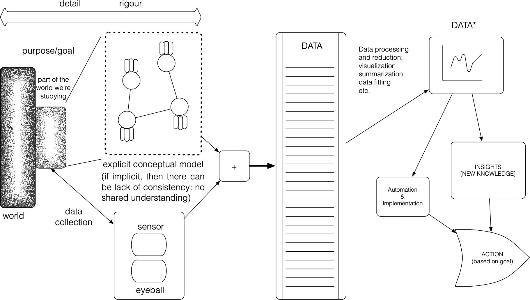
Figure 13.2: A schematic diagram of systems thinking as it applies to a general problem (J. Schellinck).
Conceptual models do not necessarily attempt to capture specific behaviours, but they emphasize the possible states of the system: the focus is on object types, not on specific instances, with abstraction as the ultimate objective.
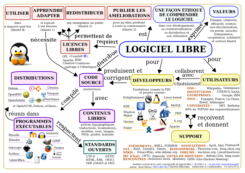
Figure 13.3: A conceptual model of the ‘free software’ system (in French) [35].
Conceptual modeling is not an exact science – it is more about making internal conceptual models explicit and tangible, and providing data analysis teams with the opportunity to examine and explore their ideas and assumptions. Attempts to formalize the concept include (see Figure 13.4):
Universal Modeling Language (UML);
Entity Relationship Models (ER), generally connected to relational databases.
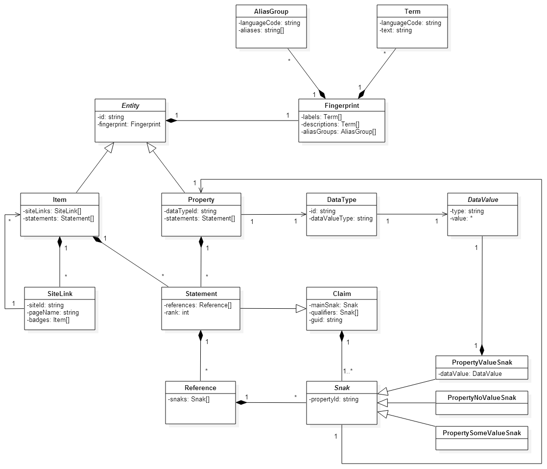
.png)
Figure 13.4: Examples of UML diagram (Wikibase Data Model, on the left [36]) and ER conceptual map (on the right [37]).
In practice, we must first select a system for the task at hand, then generate a conceptual model that encompasses:
relevant and key objects (abstract or concrete);
properties of these objects, and their values;
relationships between objects (part-whole, is-a, object-specific, one-to-many), and
relationships between properties across instances of an object type.
A simplistic example describing a supposed relationship between a presumed cause (hours of study) and a presumed effect (test score) is shown below:
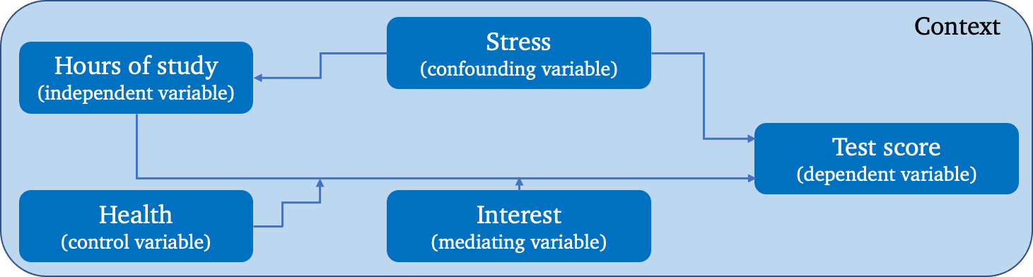
Figure 13.5: A simple conceptual model.
13.2.2.4 Relating the Data to the System
From a pragmatic perspective, stakeholders and analysts alike need to know if the data which has been collected and analyzed will be useful to understand the system.
This question can best be answered if we understand:
how the data is collected;
the approximate nature of both data and system, and
what the data represents (observations and features).
Is the combination of system and data sufficient to understand the aspects of the world under consideration? Once again, this is difficult to answer in practice.
Contextual knowledge can help, but if the data, the system, and the world are out of alignment, any data insight drawn from mathematical, ontological, programmatical, or data models of the situation might ultimately prove useless.
13.2.3 Cognitive Biases
Adding to the challenge of building good conceptual models and using these to interpret the data is the fact that we are all vulnerable to a vast array of cognitive biases, which influence both how we construct our models and how we look for patterns in the data.
These biases are difficult to detect in the spur of the moment, but being aware of them, making a conscious effort to identify them, and setting up a clear and pre-defined set of thresholds and strategies for analysis will help reduce their negative impact. Here is a sample of such biases (taken from [38], [39]).
- Anchoring bias
causes us to rely too heavily on the first piece of information we are given about a topic; in a salary negotiation, for instance, whoever makes the first offer establishes a range of reasonable possibilities in both parties’ minds.
- Availability heuristic
describes our tendency to use information that comes to mind quickly and easily when making decisions about the future; someone might argue that climate change is a hoax because the weather in their neck of the woods has not (yet!) changed.
- Bandwagon Effect
refers to our habit of adopting certain behaviours or beliefs because many others do the same; if all analyses conducted until now have shown no association between factors \(X\) and \(Y\), we might forego testing for the association in a new dataset.
- Choice-supporting bias
causes us to view our actions in a positive light, even if they are flawed; we are more likely to sweep anomalous or odd results under the carpet when they arise from our own analyses.
- Clustering illusion
refers to our tendency to see patterns in random events; if a die has rolled five 3’s in a row, we might conclude that the next throw is more (or less) likely to come up a 3 (gambling fallacy).
- Confirmation bias
describes our tendency to notice, focus on, and give greater credence to evidence that fits with our existing beliefs; gaffes made by politicians you oppose reinforces your dislike.
- Conservation bias
occurs when we favour prior evidence over new information; it might be difficult to accept that there is an association between factors \(X\) and \(Y\) if none had been found in the past.
- Ostrich effect
describes how people often avoid negative information, including feedback that could help them monitor their goal progress; a professor might chose to not consult their teaching evaluations, for whatever reason.
- Outcome bias
refers to our tendency to judge a decision on the outcome, rather than on why it was made; the fact that analysts gave Clinton an 80% chance of winning the 2016 U.S.Presidential Election does not mean that the forecasts were wrong.
- Overconfidence
causes us to take greater risks in our daily lives; experts are particularly prone to this, as they are more convinced that they are right.
- Pro-innovation bias
occurs when proponents of a technology overvalue its usefulness and undervalue its limitations; in the end, Big Data is not going to solve all of our problems.
- Recency bias
occurs when we favour new information over prior evidence; investors tend to view today’s market as the "forever’ market and make poor decisions as a result.
- Salience Bias
describes our tendency to focus on items or information that are more noteworthy while ignoring those that do not grab our attention; you might be more worried about dying in a plane crash than in a car crash, even though the latter occurs more frequently than the former.
- Survivorship Bias
is a cognitive shortcut that occurs when a visible successful subgroup is mistaken as an entire group, due to the failure subgroup not being visible; when trying to get the full data picture, it helps to know what observations did not make it into the dataset.
- Zero-Risk Bias
relates to our preference for absolute certainty; we tend to opt for situations where we can completely eliminate risk, seeking solace in the figure of 0%, over alternatives that may actually offer greater risk reduction.
Other biases impact our ability to make informed decisions:
base rate fallacy, bounded rationality, category size bias, commitment bias, Dunning-Kruger effect, framing effect, hot-hand fallacy, IKEA effect, illusion of explanatory depth, illusion of validity, illusory correlations, look elsewhere effect, optimism effect, planning fallacy, representative heuristic, response bias, selective perception, stereotyping, etc. [38], [39].
13.3 Ethics in the Data Science Context
A lapse in ethics can be a conscious choice… but it can also be negligence. R. Schutt, C. O’Neill [40]
In most empirical disciplines, ethics are brought up fairly early in the educational process and may end up playing a crucial role in researchers’ activities. At Memorial University of Newfoundland, for instance, “proposals for research in the social sciences, humanities, sciences, and engineering, including some health-related research in these areas,” must receive approval from specific .
This could, among other cases, apply to research and analysis involving [41]:
living human subjects;
human remains, cadavers, tissues, biological fluids, embryos or foetuses;
a living individual in the public arena if s/he is to be interviewed and/or private papers accessed;
secondary use of data – health records, employee records, student records, computer listings, banked tissue – if any form of identifier is involved and/or if private information pertaining to individuals is involved, and
quality assurance studies and program evaluations which address a research question.
In our experience, data scientists and data analysts who come to the field by way of mathematics, statistics, computer science, economics, or engineering, however, are not as likely to have encountered ethical research boards or to have had formal ethics training.23 Furthermore, discussions on ethical matters are often tabled, perhaps understandably, in favour of pressing technical or administrative considerations (such as algorithm selection, data cleaning strategies, contractual issues, etc.) when faced with hard deadlines.
The problem, of course, is that the current deadline is eventually replaced by another deadline, and then by a new deadline, with the end result that the conversation may never take place. It is to address this all-too-common scenario that we take the time to discuss ethics in the data science context; more information is available in [42].
13.3.1 The Need for Ethics
When large scale data collection first became possible, there was to some extent a ‘Wild West’ mentality to data collection and use. To borrow from the old English law principle, whatever was not prohibited (from a technological perspective) was allowed.
Now, however, professional codes of conduct are being devised for data scientists [43]–[45], outlining responsible ways to practice data science – ways that are legitimate rather than fraudulent, and ethical rather than unethical.24 Although this shifts some added responsibility onto data scientists, it also provides them with protection from clients or employers who would hire them to carry out data science in questionable ways – they can refuse on the grounds that it is against their professional code of conduct.
13.3.2 What Is/Are Ethics?
Broadly speaking, ethics refers to the study and definition of right and wrong conducts. Ethics may consider what is a right or a wrong action in general, or consider how broad ethical principles are appropriately applied in more specific circumstances.
And, as noted by R.W. Paul and L. Elder, ethics is not (necessarily) the same as social convention, religious beliefs, or laws [49]; that distinction is not always fully understood. The following influential ethical theories are often used to frame the debate around ethical issues in the data science context:
Kant’s golden rule: do unto others as you would have them do unto you;
Consequentialism: the end justifies the means;
Utilitarianism: act in order to maximize positive effect;
Moral Rights: act to maintain and protect the fundamental rights and privileges of the people affected by actions;
Justice: distribute benefits and harm among stakeholders in a fair, equitable, or impartial way.
In general, it is important to remember that our planet’s inhabitants subscribe to a wide variety of ethical codes, including also:
Confucianism, Taoism, Buddhism, Shinto, Ubuntu, Te Ara Tika (Maori), First Nations Principles of OCAP, various aspects of Islamic ethics, etc.
It is not too difficult to imagine contexts in which either of these (or other ethical codes, or combinations thereof) would be better-suited to the task at hand – the challenge is to remember to inquire and to heed the answers.
13.3.3 Ethics and Data Science
How might these ethical theories apply to data analysis? The (former) University of Virginia’s Centre for Big Data Ethics, Law and Policy suggested some specific examples of data science ethics questions [50]:
who, if anyone, owns data?
are there limits to how data can be used?
are there value-biases built into certain analytics?
are there categories that should never be used in analyzing personal data?
should data be publicly available to all researchers?
The answers may depend on a number of factors, not least of which being who is actually providing them. To give you an idea of some of the complexities, let us consider the first of those questions: who, if anyone, owns data?
In some sense, the data analysts who transform the data’s potential into usable insights are only one of the links in the entire chain. Processing and analyzing the data would be impossible without raw data on which to work, so the data collectors also have a strong ownership claim to the data.
But collecting the data can be a costly endeavour, and it is easy to imagine how the sponsors or employers (who made the process economically viable in the first place) might feel that the data and its insights are rightfully theirs to dispose of as they wish.
In some instances, the law may chime in as well. One can easily include other players: in the final analysis, this simple question turns out to be far from easily answered. This also highlights some of the features of the data analysis process: there is more to data analysis than just data analysis. The answer is not easily forthcoming, and may change from one case to another.
A similar challenge arises in regards to open data, where the “pro” and “anti” factions both have strong arguments (see [51]–[53], and [54] for a science-fictional treatment of the transparency-vs.-secrecy/security debate).
A general principle of data analysis is to eschew the anecdotal in favour of the general – from a purely analytical perspective, too narrow a focus on specific observations can end up obscuring the full picture (a vivid illustration can be found in [55]).
But data points are not solely marks on paper or electro-magnetic bytes on the cloud. Decisions made on the basis of data science (in all manners of contexts, from security, to financial and marketing context, as well as policy) may affect living beings in negative ways. And it can not be ignored that outlying/marginal individuals and minority groups often suffer disproportionately at the hands of so-called evidence-based decisions [56]–[58].
13.3.4 Guiding Principles
Under the assumption that one is convinced of the importance of proceeding ethically, it could prove helpful to have a set of guiding principles to aid in these efforts.
In his seminal science fiction series about positronic robots, Isaac Asimov introduced the now-famous Laws of Robotics, which he believed would have to be built-in so that robots (and by extension, any tool used by human beings) could overcome humanity’s Frankeinstein’s complex (the fear of mechanical beings) and help rather than hinder human social, scientific, cultural, and ecomomic activities [59]:
1. A robot may not injure a human being or, through inaction, allow a human being to come to harm.
2. A robot must obey the orders given to it by human beings, except where such orders would conflict with the 1st Law.
3. A robot must protect its own existence as long as such protection does not conflict with the 1st and 2nd Law.
Had they been uniformly well-implemented and respected, the potential for story-telling would have been somewhat reduced; thankfully, Asimov found entertaining ways to break the Laws (and to resolve the resulting conflicts) which made the stories both enjoyable and insightful.
Interestingly enough, he realized over time that a Zeroth Law had to supersede the First in order for the increasingly complex and intelligent robots to succeed in their goals. Later on, other thinkers contributed a few others, filling in some of the holes.
Asimov’s (expanded) Laws of Robotics:
00. A robot may not harm sentience or, through inaction, allow sentience to come to harm.
0. A robot may not harm humanity, or, through inaction, allow humanity to come to harm, as long as this action/inaction does not conflict with the 00th Law.
1. A robot may not injure a human being or, through inaction, allow a human being to come to harm, as long as this does not conflict with the 00th or the 0th Law.
2. A robot must obey the orders given to it by human beings, except where such orders would conflict with the 00th, the 0th or the 1st Law.
3. A robot must protect its own existence as long as such protection does not conflict with the 00th, the 0th, the 1st or the 2nd Law.
4. A robot must reproduce, as long as such reproduction does not interfere with the 00th, the 0th, the 1st, the 2nd or the 3rd Law.
5. A robot must know it is a robot, unless such knowledge would contradict the 00th, the 0th, the 1st, the 2nd, the 3rd or the 4th Law.]
We cannot speak for the validity of these laws for robotics (a term coined by Asimov, by the way), but we do find the entire set satisfyingly complete.
What does this have to do with data science? Various thinkers have discussed the existence and potential merits of different sets of Laws ([60]) – wouldn’t it be useful if there were Laws of Analytics, moral principles that could help us conduct data science ethically?
13.3.4.1 Best Practices
Such universal principles are unlikely to exist, but best practices have nonetheless be suggested over the years.
- “Do No Harm”
Data collected from an individual should not be used to harm the individual. This may be difficult to track in practice, as data scientists and analysts do not always participate in the ultimate decision process.
- Informed Consent
Covers a wide variety of ethical issues, chief among them being that individuals must agree to the collection and use of their data, and that they must have a real understanding of what they are consenting to, and of possible consequences for them and others.
- The Respect of “Privacy”
This principle is dearly-held in theory, but it is hard to adhere to it religiously with robots and spiders constantly trolling the net for personal data. In the Transparent Society, D. Brin (somewhat) controversially suggests that privacy and total transparency are closely linked [52]:
"And yes, transparency is also the trick to protecting privacy, if we empower citizens to notice when neighbors [sic] infringe upon it. Isn’t that how you enforce your own privacy in restaurants, where people leave each other alone, because those who stare or listen risk getting caught?’
- Keeping Data Public
Another aspect of data privacy, and a thornier issue – should some data be kept private? Most? All? It is fairly straightforward to imagine scenarios where adherence to the principle of public data could cause harm to individuals (revealing the source of a leak in a country without where the government routinely jails members of the opposition, say), contradicting the first principle against causing harm. But it is just as easy to imagine scenarios where keeping data private would have a similar effect.
- Opt-in/Opt-out
Informed consent requires the ability to not consent, i.e. to opt out. Non-active consent is not really consent.
- Anonymize Data
Identifying fields should be removed from the dataset prior to processing and analysis. Let any temptation to use personal information in an inappropriate manner be removed from the get-go, but be aware that this is easier said than done, from a technical perspective.
- Let the Data Speak
It is crucial to absolutely restrain one’s self from cherry-picking the data. Use all of it in some way or another; validate your analysis and make sure your results are repeatable.
13.3.5 The Good, the Bad, and the Ugly
Data projects could whimsically be classified as good, bad or ugly, either from a technical or from an ethical standpoint (or both). We have identified instances in each of these classes (of course, our own biases are showing):
good projects increases knowledge, can help uncover hidden links, and so on: [14]–[16], [20], [23], [24], [30], [61]–[68]
bad projects, if not done properly, can lead to bad decisions, which can in turn decrease the public’s confidence and potentially harm some individuals: [17], [21], [28], [29], [55]
ugly projects are, flat out, unsavoury applications; they are poorly executed from a technical perspective, or put a lot of people at risk; these (and similar approaches/studies) should be avoided: [26], [27], [56]–[58], [69]
13.4 Analytics Workflow
An overriding component of the discussion so far has been the importance of context. And although the reader may be eager at this point to move into data analysis proper, there is one more context that should be considered first – the project context.
We have alluded to the idea that data science is much more than simply data analysis and this is apparent when we look at the typical steps involved in a data science project. Inevitably, data analysis pieces take place within this larger project context, as well as in the context of a larger technical infrastructure or pre-existing system.
13.4.1 The “Analytical” Method
As with the scientific method, there is a “step-by-step” guide to data analysis:
statement of objective
data collection
data clean-up
data analysis/analytics
dissemination
documentation
Notice that data analysis only makes up a small segment of the entire flow.
In practice, the process often end up being a bit of a mess, with steps taken out of sequence, steps added-in, repetitions and re-takes (see Figure 13.6).
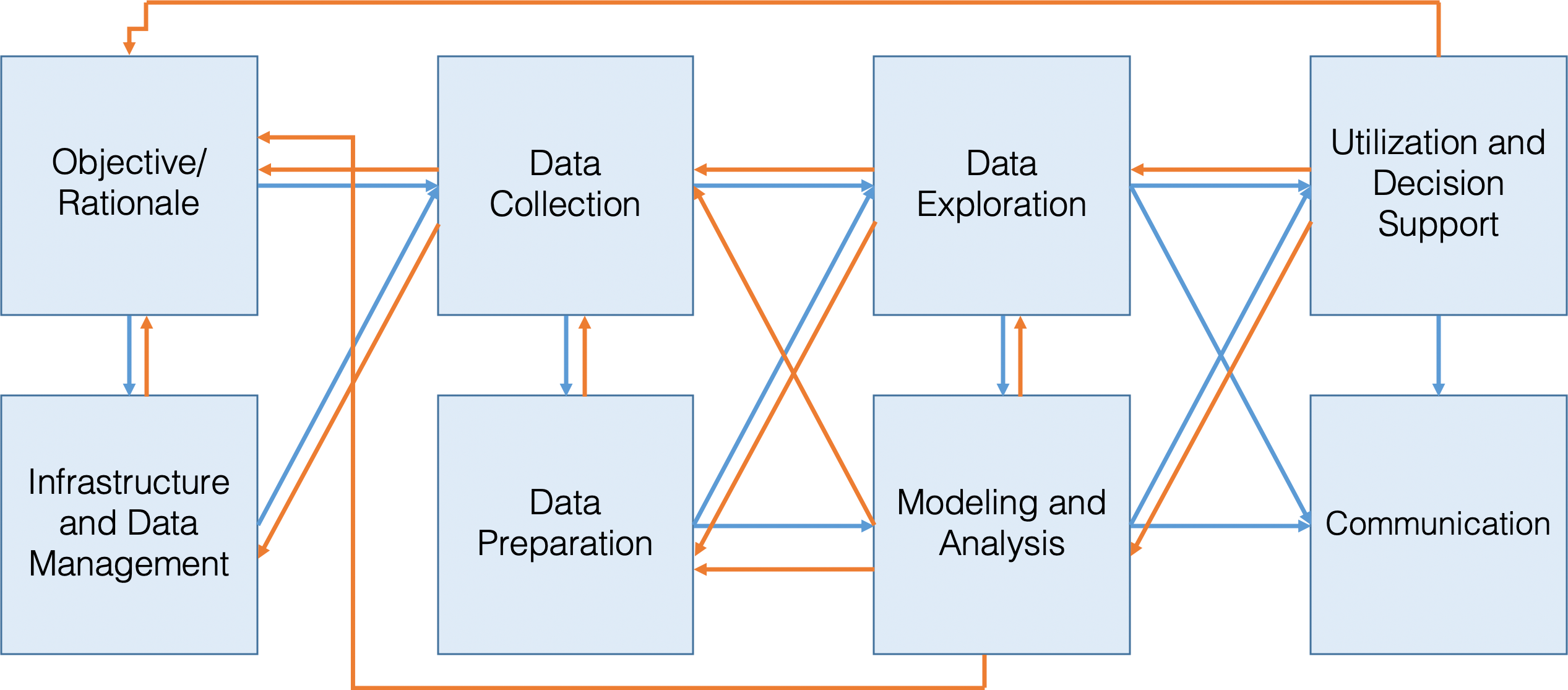
Figure 13.6: The reality of the analytic workflow – it is definitely not a linear process! [peronsal file].
And yet… it tends to work on the whole, if conducted correctly.
J. Blitzstein and H. Pfister (who teach a well-rated data science course at Harvard) provide their own workflow diagram, but the similarities are easy to spot (see Figure 13.7).
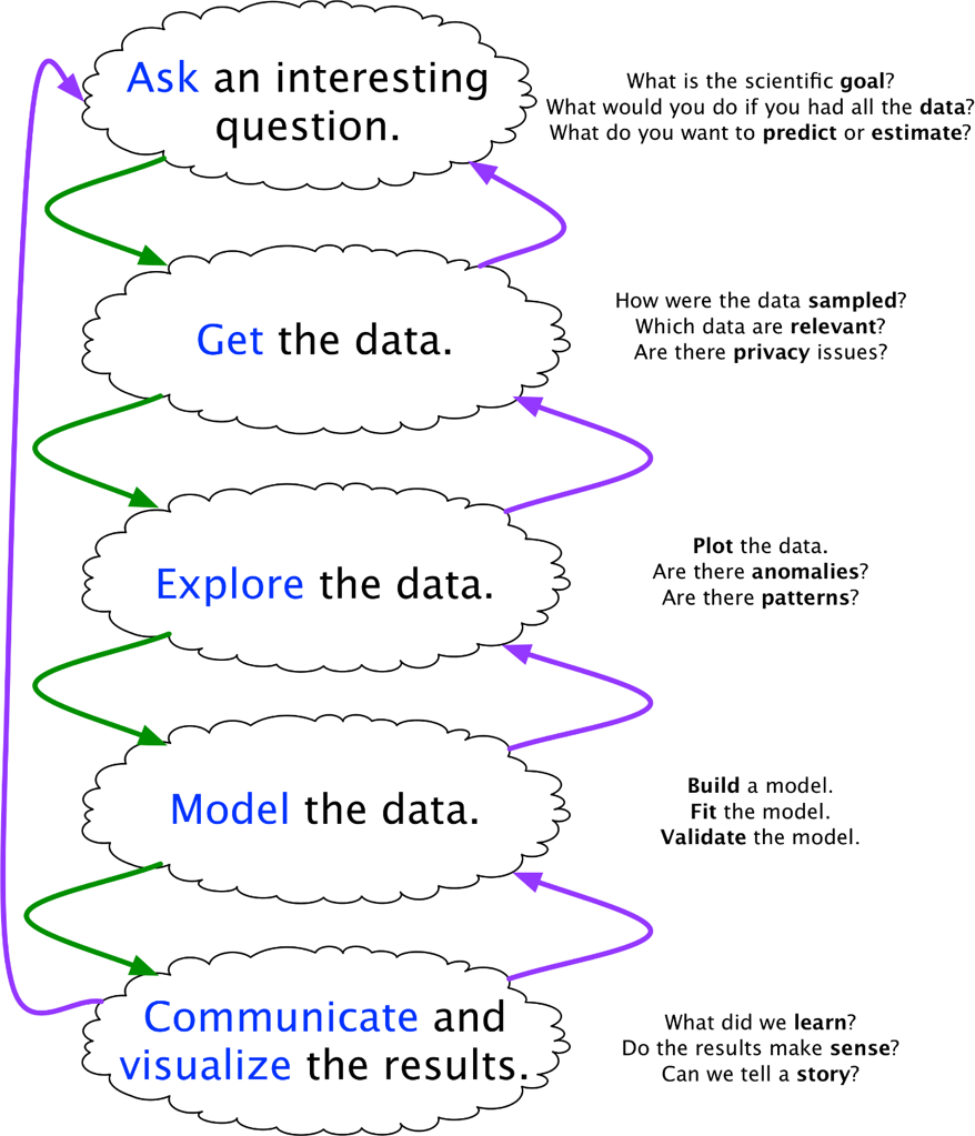
Figure 13.7: Blitzstein and Pfister’s data science workflow [reference lost].
The Cross Industry Standard Process, Data Mining is another such framework, with projects consisting of 6 steps:
business understanding
data understanding
data preparation
modeling
evaluation
deployment
The process is iterative and interactive – the dependencies are highlighted in Figure 13.8.
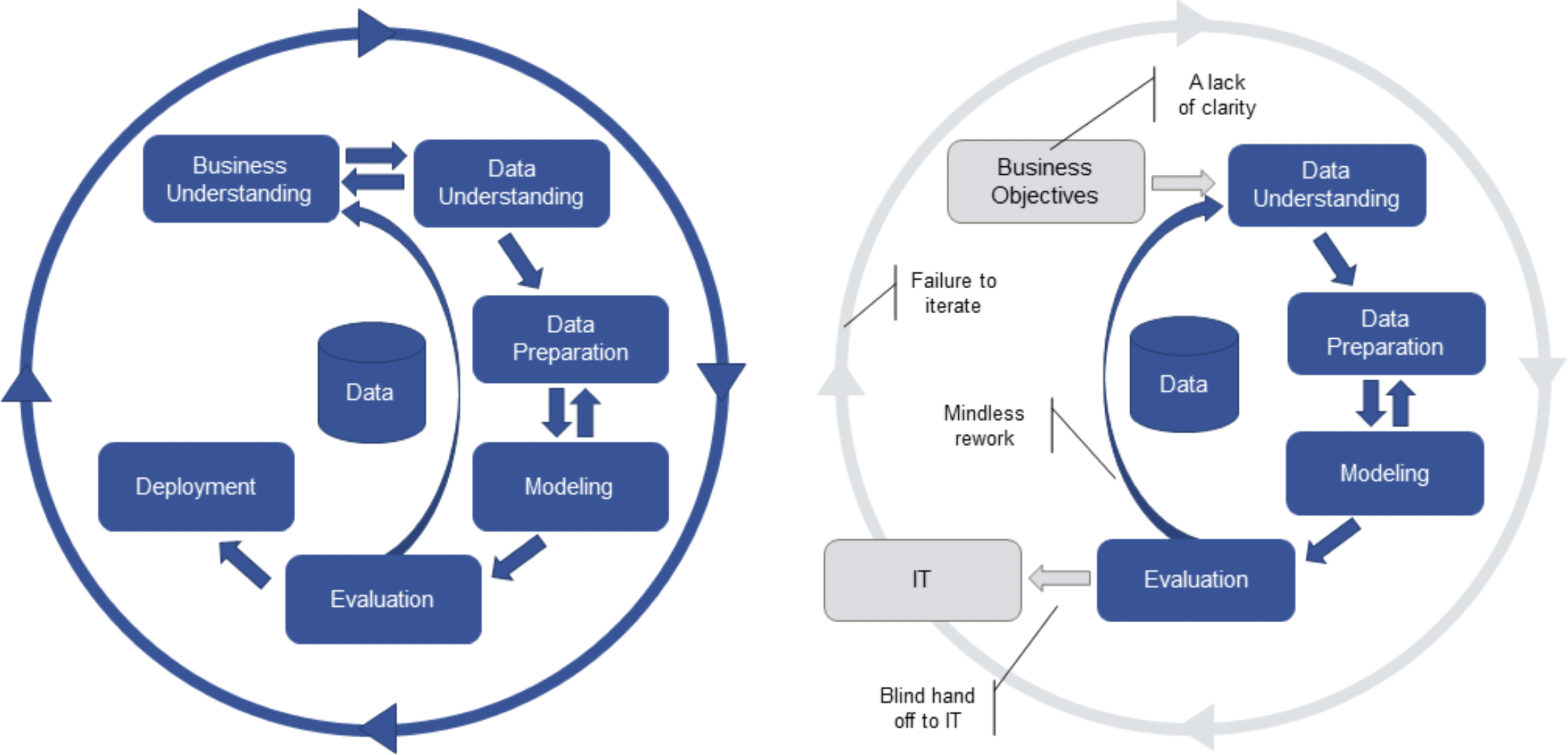
Figure 13.8: Theoretical (on the left) and corrupted (on the righ) CRISP-DM processes [70].
In practice, data analysis is often corrupted by:
lack of clarity;
mindless rework;
blind hand-off to IT, and
failure to iterate.
CRISP-DM has a definite old-hat flavour (as witnessed by the use of the outdated expression “data mining”), but it can be useful to check off its sub-components, if only as a sanity check.
- Business Understanding
understanding the business goal
assessing the situation
translating the goal in a data analysis objective
developing a project plan
- Data Understanding
considering data requirements
collecting and exploring data
- Data Preparation
selection of appropriate data
data integration and formatting
data cleaning and processing
- Modeling
selecting appropriate techniques
splitting into training/testing sets
exploring alternatives methods
fine tuning model settings
- Evaluation
evaluation of model in a business context
model approval
- Deployment
reporting findings
planning the deployment
deploying the model
distributing and integrating the results
developing a maintenance plan
reviewing the project
planning the next steps
All these approaches have a common core: data science projects are iterative and (often) non-sequential.
Helping the clients and/or stakeholders recognize this central truth will make it easier for analysts and consultants to plan the data science process and to obtain actionable insights for organizations and sponsors.
The main take-away from this section, however, is that there is a lot of real estate in the process before we can even start talking about modeling and analysis – in truth, data analysis is not solely about data analysis.
13.4.2 Data Collection, Storage, Processing, and Modeling
Data enters the data science pipeline by first being collected. There are various ways to do this:
data may be collected in a single pass;
it may be collected in batches, or
it may be collected continuously.
The mode of entry may have an impact on the subsequent steps, including on how frequently models, metrics, and other outputs are updated.
Once it is collected, data must be stored. Choices related to storage (and processing) must reflect:
how the data is collected (mode of entry);
how much data there is to store and process (small vs. big), and
the type of access and processing that will be required (how fast, how much, by whom).
Unfortunately, stored data may go stale (both figuratively, as in addresses no longer accurate, names having changed, etc., and literally, as in physical decay of the data and storage space); regular data audits are recommended.
The data must be processed before it can be analyzed. This is discussed in detail in Data Preparation, but the key point is that raw data has to be converted into a format that is amenable to analysis, by
identifying invalid, unsound, and anomalous entries;
dealing with missing values;
transforming the variables and the datasets so that they meet the requirements of the selected algorithms.
In contrast, the analysis step itself is almost anti-climactic – simply run the selected methods/algorithms on the processed data. The specifics of this procedure depend, of course, on the choice of method/algorithm.
We will not yet get into the details of how to make that choice25, but data science teams should be familiar with a fair number of techniques and approaches:
data cleaning
descriptive statistics and correlation
probability and inferential statistics
regression analysis (linear and other variants)
survey sampling
bayesian analysis
classification and supervised learning
clustering and unsupervised learning
anomaly detection and outlier analysis
time series analysis and forecasting
optimization
high-dimensional data analysis
stochastic modeling
distributed computing
etc.
These only represent a small slice of the analysis pie; it is difficult to imagine that any one analyst/data scientist could master all (or even a majority of them) at any moment, but that is one of the reasons why data science is a team activity (more on this in Roles and Responsibilities).
13.4.3 Model Assessment and Life After Analysis
Before applying the findings from a model or an analysis, one must first confirm that the model is reaching valid conclusions about the system of interest.
All analytical processes are, by their very nature, reductive – the raw data is eventually transformed into a small(er) numerical outcome (or summary) by various analytical methods, which we hope is still related to the system of interest (see Conceptual Frameworks for Data Work).
Data science methodologies include an assessment (evaluation, validation) phase. This does not solely provide an analytical sanity check (i.e., are the results analytically compatible with the data?); it can be used to determine when the system and the data science process have stepped out of alignment. Note that past successes can lead to reluctance to re-assess and re-evaluate a model (the so-called tyranny of past success); even if the analytical approach has been vetted and has given useful answers in the past, it may not always do so.
At what point does one determine that the current data model is out-of-date? At what point does one determine that the current model is no longer useful? How long does it take a model to react to a conceptual shift?26 This is another reason why regular audits are recommended – as long as the analysts remain in the picture, the only obstacle to performance evaluation might be the technical difficulty of conducting said evaluation.
When an analysis or model is ‘released into the wild’ or delivered to the client, it often take on a life of its own. When it inevitably ceases to be current, there may be little that (former) analysts can do to remedy the situation.
Data analysts and scientists rarely have full (or even partial) control over model dissemination; consequently, results may be misappropriated, misunderstood, shelved, or failed to be updated, all without their knowledge. Can conscientious analysts do anything to prevent this?
Unfortunately, there is no easy answer, short of advocating for analysts and consultants to not solely focus on data analysis – data science projects afford an opportunity to educate clients and stakeholders as to the importance of these auxiliary concepts.
Finally, because of analytic decay, it is crucial not to view the last step in the analytical process as a static dead end, but rather as an invitation to return to the beginning of the process.
13.4.4 Automated Data Pipelines
In the service delivery context, the data analysis process is typically implemented as an automated data pipeline, to enable the analysis process to occur repeatedly and automatically.
Data pipelines are usually consist of 9 components (5 stages and 4 transitions, as in Figure @ref(fig:automated_pipeline)):
data collection
data storage
data preparation
data analysis
data presentation
Each of these components must be designed and then implemented. Typically, at least one pass of the data analysis process has to be done manually before the implementation is completed.
We will return to this topic in Structuring and Organizing Data).
13.5 Non-Technical Aspects of Data Work
The main skill set of a data scientist is the ability to apply quantitative methods to business problems in order to obtain actionable insight.
As mentioned previously, it is impossible for any given individual to have expertise in every field of mathematics, statistics, and computer science. In our experience, the best outputs are achieved when a small team of data scientists and consultants possesses expertise in 2 or 3 areas, a decent understanding of related disciplines, and a passing knowledge in a variety of other domains.
This requires analysts to:
keep up with trends;
implement knowledge redundancies on the team;
become conversant in non-expertise areas, and
to know where to find information (online, in books, or from external resources).
In this section, however, we focus on the non-technical aspects of quantitative work. Note that these are not just bells and whistles; analysts that neglect them will see their project fail, no matter how cleverly their analyses were conducted (see [71] for more details).
13.5.1 The Data Science Framework
The perfect data scientist is both reliable and extremely skilled; but in a pinch, it’s much preferable to be merely good and reliable than to be great but flaky. (B. Rayfield, paraphrased)
Data scientists’ duties could include some of the following:
making recommendations to improve products or services;
implementing solutions;
breathing new life into a failing project;
training colleagues,
etc.
More specifically, good data scientists are expected to:
have business acumen;
learn how to manage projects from inception to completion while working with various people, on various projects, and understanding that these people could also be working on various projects;
be able to slot into various team roles, recognize when to take the lead and when to take a backseat, when to focus on building consensus and when to focus on getting the work done;
seek personal and professional development, which means that the learning never stops;
always display professionalism (externally and internally), take ownership of failures and share the credit in successes, treat colleagues, stakeholders, and clients with respect, and demand respect for teammates, stakeholders, and clients as well;
act according to their ethical system;
hone their analytical, predictive, and creative thinking skills;
rely on their emotional intelligence, as it is not sufficient to have a high IQ and recognize stated and tacit colleagues’ and clients’ needs, and
communicate effectively with clients, stakeholders, and colleagues, to manage projects and deliver results.
13.5.2 Multiple “I”s Approach to Quantitative Work
While technical and quantitative proficiency (or expertise) is of course necessary to do good quantitative work, it is not sufficient – optimal real-world solutions may not always be the optimal academic or analytical solutions. This can be a difficult pill to swallow for individuals that have spent their entire education on purely quantitative matters.
The analysts’ focus should then shift to the delivery of useful analyses, obtained via the Multiple “I”s approach to data science:
intuition – understanding the data and the analysis context;
initiative – establishing an analysis plan;
innovation – searching for new ways to obtain results, if required;
insurance – trying more than one approach, even when the first approach worked;
interpretability – providing explainable results;
insights – providing actionable results;
integrity – staying true to the analysis objectives and results;
independence – developing self-learning and self-teaching skills;
interactions – building strong analyses through (often multi-disciplinary) teamwork;
interest – finding and reporting on interesting results;
intangibles – putting a bit of yourself in the results and deliverables, and thinking “outside the box”;
inquisitiveness – not simply asking the same questions over and over again.
Data scientists should not only heed the Multiple “I”s at the delivery stage of the process – they can inform every other stage leading to it.
13.5.3 Roles and Responsibilities
To leverage Big Data efficiently, an organization needs business analysts, data scientists, and big data developers and engineers. [De Mauro, Greco, Grimaldi [73]]
A data analyst or a data scientist (in the singular) is unlikely to get meaningful results – there are simply too many moving parts to any data project.
Successful projects require teams of highly-skilled individuals who understand the data, the context, and the challenges faced by their teammates.27
Depending on the scope of the project, the team’s size could vary from a few to several dozens (or more!) – it is typically easier to manage small-ish teams (with 1-4 members, say).

Figure 13.9: A data science team in action, warts and all [Meko Deng, 2017].
Our experience as consultants and data scientists has allowed us to identify the following quantitative/data work roles.28
- Project Managers / Team Leads
have to understand the process to the point of being able to recognize whether what is being done makes sense, and to provide realistic estimates of the time and effort required to complete tasks. Team leads act as interpreters between the team and the clients/stakeholders, and advocate for the team.29 They might not be involved with the day-to-day aspects of the projects but are responsible for the project deliverables.
- Domain Experts / SMEs
are, quite simply, authorities in a particular area or topic. Not “authority” in the sense that their word is law, but rather, in the sense that they have a comprehensive understanding of the context of the project, either from the client/stakeholder side, or from past experience. SMEs can guide the data science team through the unexpected complications that arise from the disconnect between data science team and the people “on-the-ground”, so to speak.
- Data Translators
have a good grasp on the data and the data dictionary, and help SMEs transmit the underlying context to the data science team.
- Data Engineers / Database Specialists
work with clients and stakeholders to ensure that the data sources can be used down the line by the data science team. They may participate in the analyses, but do not necessarily specialize in esoteric methods and algorithms. Most data science activities require the transfer of some client data to the analysis team. In many instances, this can be as simple as sending a
.csvfile as an e-mail attachment. In other instances, there are numerous security and size issues that must be tackled before the team can gain access to the data.- Data Scientists
are team members who work with the processed data to build sophisticated models that provide actionable insights. They have a sound understanding of algorithms and quantitative methods, and of how they can be applied to a variety of data scenarios. They typically have 2 or 3 areas of expertise and can be counted on to catch up on new material quickly.
- Computer Engineers
design and build computer systems and other similar devices. They are also involved in software development, which is frequently used to deploy data science solutions.
- Artificial Intelligence/Machine Learning Quality Assurance/Quality Control (AI/ML QA/QC) Specialists
design testing plans for solutions that implement AI/ML models; in particular, they should help the data science team determine whether the models are able to learn.
- Communication Specialists
are team members who can communicate the actionable insights to managers, policy analysts, decision-makers and other stake holders. They participate in the analyses, but do not necessarily specialize in esoteric methods and algorithms. They should keep on top of popular accounts of quantitative results. They are often data translators, as well.
Another complication is provided by the fact that data science projects can be downright stressful. In an academic environment, the pace is significantly looser, but
deadlines still exist (exams, assignments, theses),
work can pile up (multiple courses, TAs, etc.)
In the workplace, there are two major differences:
a data science project can only really receive 1 of 3 “grades”: A+ (exceeded expectations), A- (met expectation), or F (didn’t meet expectations);
while project quality is crucial, so is timeliness – missing a deadline is just as damaging as turning in uninspired or flawed work; perfect work delivered late may cost the client a sizeable amount of money.
Sound project management and scheduling can help alleviate some of the stress related to these issues. These are the purview of project managers and team leads, as is the maintenance of the quality of team interactions, which can make or break a project:
treat colleagues/clients with respect AT ALL TIMES – that includes emails, Slack conversations, watercooler conversations, meetings, progress reports, etc.;
keep interactions cordial and friendly – you do not have to like your teammates, but you are all pulling in the same direction;
keep the team leader/team abreast of developments and hurdles – delays may affect the project management plan in a crucial manner (plus your colleagues might be able to offer suggestions), and
respond to requests and emails in a timely manner (within reason, of course).
13.5.4 Non-Technical Data Cheat Sheet
We will end this section with a 12-point TL;DR (too long; didn’t read) snippet that summarizes the profession. These were collected (sometimes rather painfully) throughout the years (see [72] for more details).
Business solutions are not always academic solutions.
The data and models don’t always support the stakeholder/client’s hopes, wants, and needs.
Timely communication is key – with the client and stakeholders, and with your team.
Data scientists need to be flexible (within reason), and willing and able to learn something new, quickly.
Not every problem calls for data science methods.
We should learn from both from our good and our bad experiences.
Manage projects and expectations.
Maintain a healthy work-life balance.
Respect the client, the project, the methods, and ther team.
Data science is not about how smart we are; it is about how we can provide actionable insight.
When what the client wants can’t be done, offer alternatives.
“There ain’t no such thing as a free lunch.”
13.6 Getting Insight From Data
With all of the appropriate context now in mind, we can finally turn to the main attraction, data analysis proper. Let us start this section with a few definitions, in order to distinguish between some of the common categories of data analysis.
What is Data Analysis?
We view finding patterns in data as being data analysis’s main goal. Alternatively, we could describe the data analysis process as using data to:
answer specific questions;
help in the decision-making process;
create models of the data;
describe or explain the situation or system under investigation;
etc.
While some practitioners include other analytical-like activities, such as testing (scientific) hypotheses, or carrying out calculations on data, we think of those as separate activities.
What is Data Science?
One of the challenges of working in the data science field is that nearly all quantitative work can be described as data science (often to a ridiculous extent).
Our simple definition paraphrase T. Kwartler: data science is the collection of processes by which we extract useful and actionable insights from data. Robinson [74] further suggests that these insights usually come via visualization and (manual) inferential analysis.
The noted data scientist H.Mason thinks of the discipline as “the working intersection of statistics, engineering, computer science, domain expertise, and”hacking" [75]).
What is Machine Learning?
Starting in the 1940s, researchers began to take seriously the idea that machines could be taught to learn, adapt and respond to novel situations.
A wide variety of techniques, accompanied by a great deal of theoretical underpinning, were created in an effort to achieve this goal.
Machine learning is typically used in a second stage, to obtain “predictions” (or “advice”), while reducing the operator’s analytical, inferential and decisional workload (although it is still present to some extent) [74].
What is Artificial/Augmented Intelligence?
The science fiction answer is that artificial intelligence is non-human intelligence that has been engineered rather than one that has evolved naturally. Practically speaking, this translates to “computers carrying out tasks that only humans can do”.
A.I. attempts to remove the need for oversight, allowing for automatic “actions” to be taken by a completely unattended system.
These goals are laudable in an academic setting, but we believe that stakeholders (and humans, in general) should not seek to abdicate all of their agency in the decision-making process; as such, we follow the lead of various thinkers and suggest further splitting A.I. into general A.I. (who would operate independently of human intelligence) and augmented intelligence (which enhances human intelligence).
13.6.1 Asking the Right Questions
Definitions aside, however, data analysis, data science, machine learning, and artificial intelligence are about asking questions and providing answers to these questions. We might ask various types of questions, depending on the situation.
Our position is that, from a quantitative perspective, there are only really three types of questions:
analytics questions
data science questions, and
quantitative methods questions.
Analytics questions could be something as simple as:
how many clicks did a specific link on my website get?
Data science questions tend to be more complex – we might ask something along the lines of:
if we know, historically, when or how often people click on links, can we predict how many people from Winnipeg will access a specific page on our website within the next three hours?
Whereas analytics-type questions are typically answered by counting things, data science-like questions are answered by using historical patterns to make predictions.
Quantitative methods questions might, in our view, be answered by making predictions but not necessarily based on historical data. We could build a model from first principles – the “physics” of the situation, as it were – to attempt to figure out what might happen.
For instance, if we thought there was a correlation between the temperature in Winnipeg and whether or not people click on the links in our website, then we might build a model that predicts “how many people from Winnipeg will access a page in the next week?”, say, by trying to predict the weather instead,30 which is not necessarily an easy task.
Analytics models do not usually predict or explain anything – they just report on the data, which is itself meant to represent the situation. A data mining or a data science model tends to be predictive, but not necessarily explanatory – it shows the existence of connections, of correlations, of links, but without explaining why the connections exist.
In a quantitative method model, we may start by assuming that we know what the links are, what the connections are – which presumably means that we have an idea as to why these connections exist31 – and then we try to explore the consequences of the existence of these connections and these links.
This leads to a singular realization that we share with new data scientists and analysts (potentially the single most important piece of advice they will receive in their quantitative career, and we are only half-joking when we say it):
not every situation calls for analytics, data science, statistical analysis, quantitative methods, machine learning, or A.I.
Take the time to identify instances where more is asked out of the data than what it can actually yield, and be prepared to warn stakeholders, as early as possible, when such a situation is encountered.
If we cannot ask the right questions of the data, of the client, of the situation, and so on, any associated project is doomed to fail from the very beginning. Without questions to answer, analysts are wasting their time, running analyses for the sake of analysis – the finish line cannot be reached if there is no finish line.
In order to help clients/stakeholders, data analysts and scientists need:
questions to answer,
questions that can be answered by the types of methods and skills at their disposal, and
answers that will be recognized as answers.
“How many clicks did this link get?” is a question that is easily answerable if we have a dataset of links and clicks, but it might not be a question that the client cares to see answered.
Data analysts and scientists often find themselves in a situation where they will ask the types of questions that can be answered with the available data, but the answers might not prove actually useful.
From a data science perspective, the right question is one that leads to actionable insights. And it might mean that old data is discared and new data is collected in order to answer it. Analysts should beware: given the sometimes onerous price tag associated to data collection, it is not altogether surprising that there will sometimes be pression from above to keep working with the available data.
Stay strong – analysis on the wrong dataset is the wrong analysis!
13.6.1.1 The Wrong Questions
Wrong questions might be:
questions that are too broad or too narrow;
questions that no amount of data could ever answer;
questions for which data cannot reasonably be obtained, etc.
One of the issues with “wrong” questions is that they do not necessarily “break the pipeline”:
in the best-case scenario, stakeholders, clients, colleagues will still recognize the answers as irrelevant.
in the worst-case scenario, policies will erroneously be implemented (or decisions made) on the basis of answers that have not been identified as misleading and/or useless.
13.6.2 Structuring and Organizing Data
Let us now resume the discussion that was cut short in What Is Data? and From Objects and Attributes to Datasets.
13.6.2.1 Data Sources
We cannot have insights from data without data. As with many of the points we have made, this may seem trivially obvious, but there are many aspects of data acquisition, structuring, and organization that have a sizable impact on what insights can be squeezed from data.
More specifically, there are a number of questions that can be considered:
why do we collect data?
what can we do with data?
where does data come from?
assuming we collect data so we can have a collection of data, what does “a collection” of data look like?
how can we describe data?
do we need to distinguish between data, information, knowledge?32
Historically, data has had three functions:
record keeping – people/societal management (!);
science – new general knowledge, and
intelligence – business, military, police, social (?), domestic (?), personal (!)
Traditionally, each of these functions has
used different sources of information;
collected different types of data, and
had different data cultures and terminologies.
As data science is an interdisciplinary field, it should come as no surprise that we may run into all of them on the same project (see Figure 13.10).
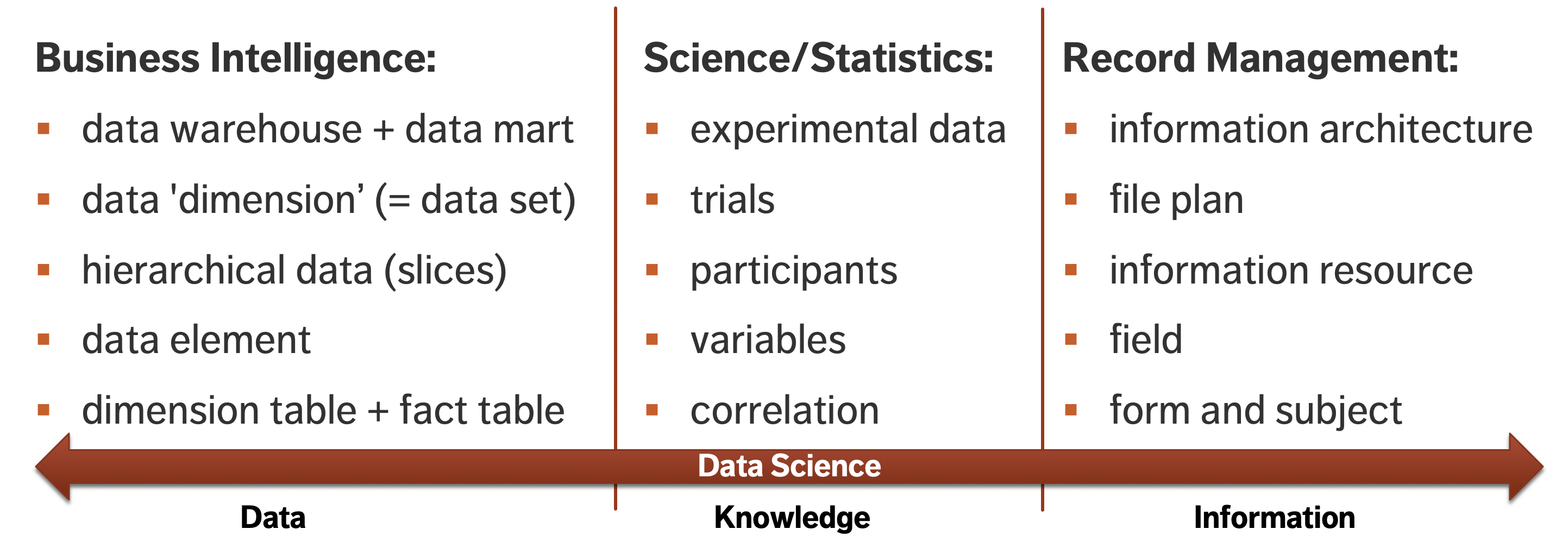
Figure 13.10: Different data cultures and terms.
Ultimately, data is generated from making observations about and taking measurements of the world. In the process of doing so, we are already imposing particular conceptualizations and assumptions on our raw experience.
More concretely, data comes from a variety of sources, including:
records of activity,
(scientific) observations,
sensors and monitoring, and,
more frequently lately, from computers themselves.
As discussed in Section The Analog/Digital Data Dichotomy, although data may be collected and recorded by handed, it is fast becoming a mostly digital phenomenon.
Computer science (and information science) has its own theoretical, fundamental viewpoint about data and information, operating over data in a fundamental sense – 1s and 0s that represent numbers, letters, etc. Pragmatically, the resulting data is now stored on computers, and is accessible through our world-wide computer network.
While data is necessarily a representation of something else, analysts should endeavour to remember that the data itself still has physical properties: it takes up physical space and requires energy to work with.
In keeping with this physical nature, data also has a shelf life – it ages over time. We use the phrase “rotten data” or “decaying data” in one of two senses:
literally, as the data storage medium might decay, but also
metaphorically, as when it no longer accurately represents the relevant objects and relationships (or even when those objects no longer exist in the same way) – compare with “analytical decay” (see Model Assessment and Life After Analysis).
Useful data must stay ‘fresh’ and ‘current’, and avoid going ‘stale’ – but that is both context- and model-dependent!
13.6.2.2 Before the Data
The various data-using disciplines share some core (systems) concepts and elements, which should resonate with the systems modeling framework previously discussed in Conceptual Frameworks for Data Work:
all objects have attributes, whether concrete or abstract;
for multiple objects, there are relationships between these objects/attributes, and
all these elements evolve over time.
The fundamental relationships include:
part–whole;
is–a;
is–a–type–of;
cardinality (one-to-one, one-to-many, many-to-many),
etc.,
while object-specific relationships include:
ownership;
social relationship;
becomes;
leads-to,
etc.
13.6.2.3 Objects and Attributes
We can examine concretely the ways in which objects have properties, relationships and behaviours, and how these are captured and turned into data through observations and measurements, via the apple and sandwich example of What Is Data?.
There, we made observations of an apple instance, labeled the type of observation we made, and provided a value describing the observation. We can further use these labels when observing other apple instances, and associate new values for these new apple instances.
Regarding the fundamental and object specified relationships, we might be able to see that:
an apple is a type of fruit,
a sandwich is part of a meal,
this apple is owned by Jen,
this sandwich becomes fuel,
etc.
It is worth noting that while this all seems tediously obvious to adult humans, it is not so from the perspective of a toddler, or an artificial intelligence. Explicitly, “understanding” requires a basic grasp of:
categories,
instances,
types of attributes,
values of attributes, and
which of these are important or relevant to a specific situation or in general terms.
13.6.2.4 From Attributes to Datasets
Were we to run around in an apple orchard, measuring and jotting down the height, width and colour of 83 different apples completely haphazardly on a piece of paper, the resulting data would be of limited value; although it would technically have been recorded, it would be lacking in structure.
We would not be able to tell which values were heights and which were widths, and which colours or which widths were associated with which heights, and vice-versa. Structuring the data using lists, tables, or even tree structures allows analysts to record and preserve a number of important relationships:
those between object types and instances, property, attribute types (sometimes also called fields, features or dimensions), and values,
those between one attribute value and another value (i.e., both of these values are connected to this object instance),
those between attribute types, in the case of hierarchical data, and
those between the objects themselves (e.g., this car is owned by this person).
Tables, also called flat files, are likely the most familiar strategy for structuring data in order to preserve and indicate relationships. In the digital age, however, we are developing increasingly sophisticated strategies to store the structure of relationships in the data, and finding new ways to work with these increasingly complex relationship structures.
Formally, a data model is an abstract (logical) description of both the dataset structure and the system, constructed in terms that can be implemented in data management software.
In a sense, data models lie halfway between conceptual models and database implementations. The data proper relates to instances; the model to object types. Ontologies provide an alternative representation of the system: simply put, they are structured, machine-readable collections of facts about a domain.33
In a sense, an ontology is an attempt to get closer to the level of detail of a full conceptual model, while keeping the whole machine-readable (see Figure 13.11 for an example).
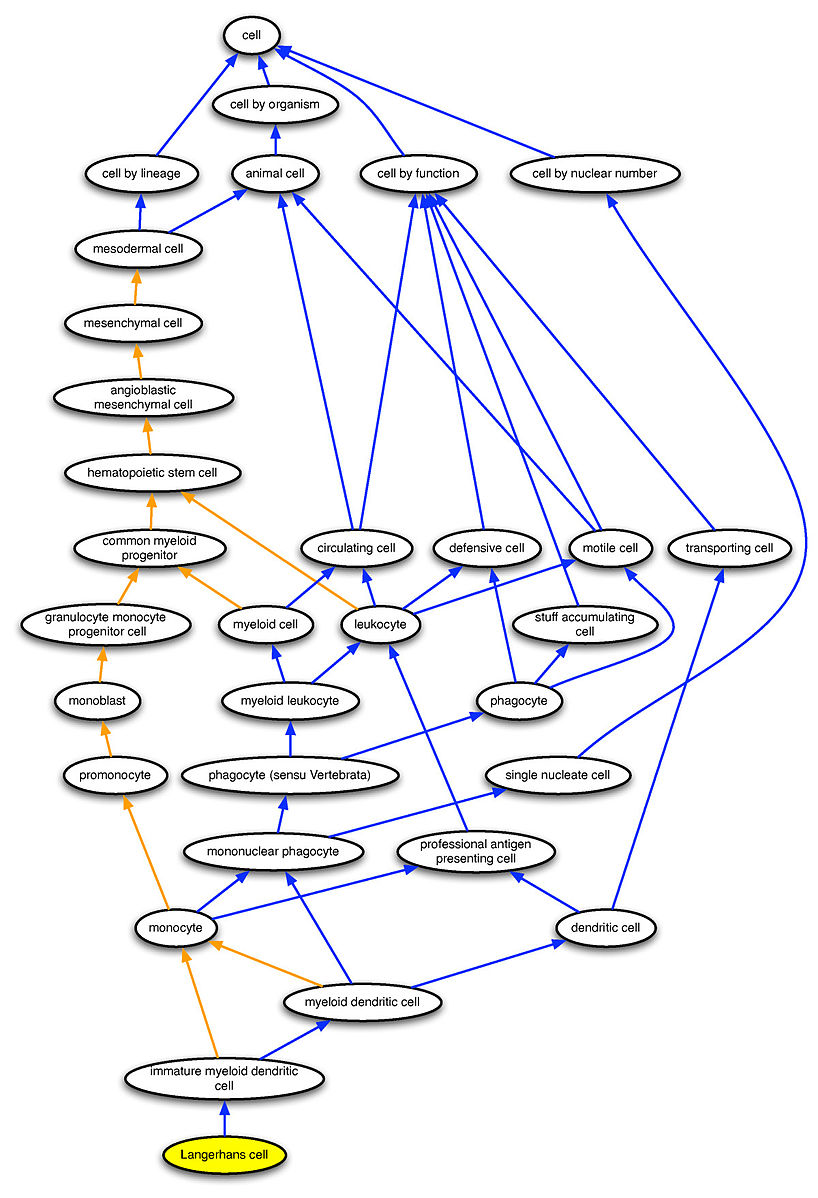
Figure 13.11: Representation of Langerhans cells in the Cell Ontology [78].
Every time we move from a conceptual model to a specific type of model (a data model, a knowledge model), we lose some information. One way to preserve as much context as possible in these new models is to also provide rich metadata – data about the data! Metadata is crucial when it comes to successfully working with and across datasets. Ontologies can also play a role here, but that is a topic for another day.
Typically data is stored in a database. A major motivator for some of the new developments in types of databases and other data storing strategies is the increasing availability of unstructured and (so-called) ‘BLOB’ data.
Structured data is labeled, organized, and discrete, with a pre-defined and constrained form. With that definition, for instance, data that is collected via an e-form that only uses drop-down menus is structured.
Unstructured data, by comparison, is not organized, and does not appear in a specific pre-defined data structure – the classical example is text in a document. The text may have to subscribe to specific syntactic and semantic rules to be understandable, but in terms of storage (where spelling mistakes and meaning are irrelevant), it is highly unstructured since any data entry is likely to be completely different from another one in terms of length, etc.
The acronym “BLOB” stands for Binary Large Object data, such as images, audio files, or general multi-media files. Some of these files can be structured-like (all pictures taken from a single camera, say), but they are usually quite unstructured, especially in multi-media modes.
Not every type of database is well-suited to all data types. Let us look at four currently popular database options in terms of fundamental data and knowledge modeling and structuring strategies:
key-value pairs (e.g. JSON);
triples (e.g. resource description framework – RDF));
graph databases, and
relational databases.
13.6.2.5 Key-Value Stores
In these, all data is simply stored as a giant list of keys and values, where the ‘key’ is a name or a label (possibly of an object) and the ‘value’ is a value associated with this key; triple stores operate on the same principle, but data is stored according to ‘subject – predicate – object’.
The following examples illustrate these concepts
The apple type – apple colour key-value store might contain
Granny Smith -- greenandRed Delicious -- red.
The person – shoe size key-value store might contain
Jen Schellinck -- women's size 7, andColin Henein -- men's size 10.
Other key-value stores: word – definition, report name – report (document file), url – webpage.
Triples stores just add a verb to the mix: person – is – age might contain
Elowyn -- is -- 18,Llewellyn -- is -- 8, andGwynneth -- is -- 4;
while object – is-colour – colour might contain
apple -- is-colour -- redandapple -- is-colour -- green.
Both strategies results in a large amount of flexibility when it comes to the ‘design’ of the data storage, and not much needs to be known about the data structure prior to implementation. Additionally, missing values do not take any space in such stores.
In terms of their implementation, the devil is in the details; note that their extreme flexibility can also be a flaw [79], and it can be difficult to query them and find the data of interest.
13.6.2.6 Graph Databases
In graph databases, the emphasis is placed on the relationships between different types of objects, rather than between an object and the properties of that object:
the objects are represented by nodes;
the relationships between these objects are represented by edges, and
objects can have a relationship with other objects of the same type (such as person is-a-sibling-of person).
They are fast and intuitive when using relation-based data, and might in fact be the only reasonable option to use in that case as traditional databases may slow to a crawl. But they are probably too specialized for non relation-based data, and they are not yet widely supported.
13.6.2.7 Relational Databases
In relational databases, data is stored in a series of tables. Broadly speaking, each table represents an object and some properties related to this object; special columns in tables connect object instances across table (the entity-relationship model diagram (ERD) of Figure 13.4 is an example of a relational database model).
For instance, a person lives in a house, which has a particular address. Sometimes that property of the house will be stored in the table that stores information about individuals; in other cases, it will make more sense to store information about the house in its own table.
The form of relational databases are driven by the cardinality of the relationships (one-to-one, one-to-many, or many-to-many). These concepts are illustrated in the cheat sheet found in Figure 13.12.
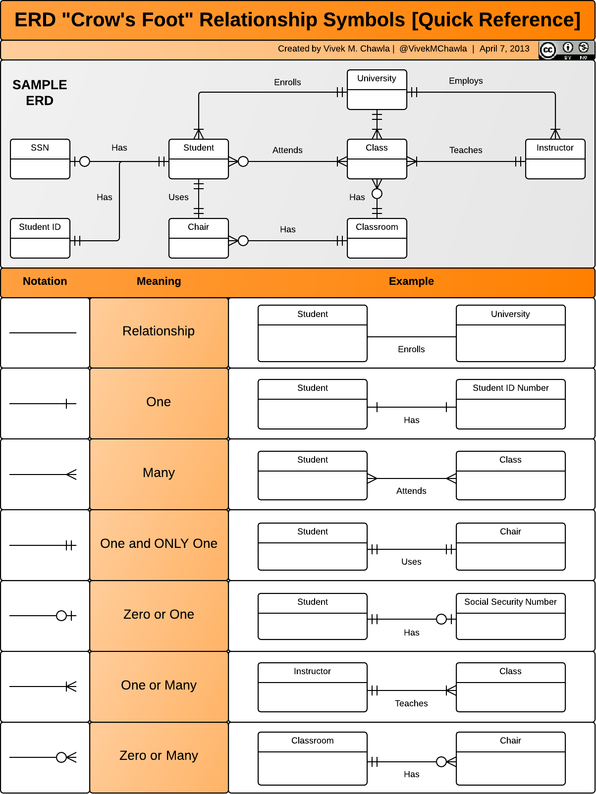
Figure 13.12: Entity-relationship model diagram ‘(so-called) ’crow’s foot’ relationship symbols cheat sheet [80].
Relational databases are widely supported and well understood, and they work well for many types of systems and use cases. Note however, that it is difficult to modify them once they have been implemented and that, despite their name, they do not really handle relationships all that well.
13.6.2.8 Spreadsheets
We have said very little about keeping data in a single giant table (spreadsheet, flatfile), or multiple spreadsheets. On the positive side, spreadsheets are very efficient when working with:
static data (e.g., it is only collected once), or
data about one particular type of object (e.g., scientific studies).
Most implementations of analytical algorithms require the data to be found in one location (such as an R data frame). Since the data will eventually need to be exported to a flatfile anyway, why not remove the middle step and work with spreadsheets in the first place?
The problem is that it is hard to manage data integrity with spreadsheets over the long term when data is collected (and processed) continuously. Furthermore, flatfiles are not ideal when working with systems involving many different types of objects and their relationships, and they are not optimzed for querying operations.
For small datasets or quick-and-dirty work, flatfiles are often a reasonable option, but analysts should look for alternatives when working on large scale projets.
All in all, we have provided very little in the way of concrete information on the topic of databases and data stores – be aware that, time and time again, projects have sunk when this aspect of the process has not been taken seriously: simply put, serious analyses cannot be conducted properly without the right data infrastructure.
13.6.2.9 Implementing a Model
In order to implement the data/knowledge model, data engineers and database specialists need access to data storage and management software. Gaining this access might be challenging for individuals or small teams as the required software traditionally runs on servers.
A server allows multiple users to access the database simultaneously, from different client programs. The other side of the coin is that servers make it difficult to ‘play’ with the database.
User-friendly embedded database software (by opposition to client-server database engines) such as SQLite can help overcome some of these obstacles. Data management software lets human agents interact easily with their data – in a nutshell, they are a human–data interface, through which
data can be added to a data collection,
subsets can be extracted from a data collection based on certain filters/criteria, and
data can be deleted from (or edited in) a data collection.
But tempora mutantur, nos et mutamur in illis34 – whereas we used to speak of:
databases and database management systems;
data warehouses (data management system designed to enable analytics);
data marts (used to retrieve client-facing data, usually oriented to a specific business line or team);
Structured Query Language (SQL, a commonly-used programming language that helps manage (and perform operations on) relational databases),
we now speak of (see [81]):
data lakes (centralized repository in which to store structured/unstructured data alike);
data pools (a small collection of shared data that aspires to be a data lake, someday);
data swamps (unstructured, ungoverned, and out of control data lake in which data is hard to find/use and is consumed out of context, due to a lack of process, standards and governance);
database graveyards (where databases go to die?);
and data might be stored in non-traditional data structures, such as
Popular NoSQL database software include: ArangoDB, MongoDB, Redis,Amazon DynamoDB, OrientDB, Azure CosmosDB, Aerospike, etc.
Once a logical data model is complete, we need only:
instantiate it in the chosen software;
load the data, and
query the data.
Traditional relational databases use SQL; other types of databases either use other query languages (AQL, semantic engines, etc.) or rely on bespoke (tailored) computer programs (e.g. written in R, Python, etc.).
Once a data collection has been created, it must be managed, so that the data remains accurate, precise, consistent, and complete. Databases decay, after all; if a data lake turns into a data swamp, it will be difficult to squeeze usefulness out of it!
13.6.2.10 Data and Information Architectures
There is no single correct structure for a given collection of data (or dataset).
Rather, consideration must be given to:
the type of relationships that exist in the data/system (and are thought to be important);
the types of analysis that will be carried out, and
the data engineering requirements relating to the time and effort required to extract and work with the data.
The chosen structure, which stores and organizes the data, is called the data architecture; designing a specific architecture for a data collection is a necessary part of the data analysis process. The data architecture is typically embedded in the larger data pipeline infrastructure described in Automated Data Pipelines.
As another example, automated data pipelines in the service delivery context are usually implemented with 9 components (5 stages, and 4 transitions, as in Figure 13.13):
data collection
data storage
data preparation
data analysis
data presentation
Note that model validation could be added as a sixth stage, to combat model “drift”.
By analogy with the human body, the data storage component, which houses the data and its architecture, is the “heart” of the pipeline (the engine that makes the pipeline go), whereas the data analysis component is its “brain.”35
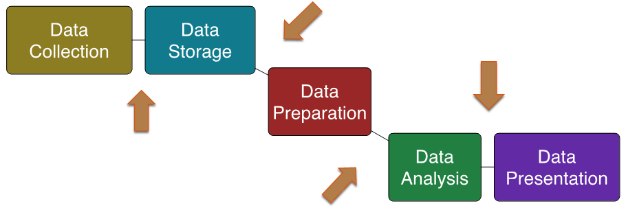
Figure 13.13: An implemented automated pipeline; note the transitions between the 5 stages.
Most analysts are familiar with mathematical and statistical models which are implemented in the data analysis component; data models tend to get constructed separately from the analytical models, at the data storage phase. This separation can be problematic if the analytical model is not compatible with the data model. As an example, if an analyst needs a flatfile (with variables represented as columns) to feed into an algorithm implemented in R, say.
If the data comes from forms with various fields stored in a relational database, the discrepancy could create difficulties on the data preparation side of the process.
Building both the analytical model and the data model off of a common conceptual model might help the data science team avoid such quandaries.
In essence, the task is to structure and organize both data and knowledge so that it can be:
stored in a useful manner;
added to easily;
usefully and efficiently extracted from that store (the “extract-transform-load” (ETL) paradigm), and
operated over by humans and computers alike (programs, bots, A.I.) with minimal external modification.
13.6.3 Basic Data Analysis Techniques
Business Intelligence (BI) has evolved over the years:
we started to recognize that data could be used to gain a competitive advantage at the end of the 19th century;
the 1950s saw the first business database for decision support;
in the 1980s and 1990s, computers and data became increasingly available (data warehouses, data mining);
in the 2000s, the trend was to take business analytics out of the hands of data miners (and other specialists) and into the hands of domain experts.
Now, big data and specialized techniques have arrived on the scene, as have data visualization, dashboards, and software-as-service.
Historically, BI has been one of the streams contributing to modern day data science;
system of interest: the commercial realm, specifically, the market of interest;
sources of data: transaction data, financial data, sales data, organizational data;
goals: provide awareness of competitors, consumers and internal activity and use this to support decision making;
culture and preferred techniques: datamarts, key performance indicators, consumer behaviour, slicing and dicing, business ‘facts’.
But no matter the realm in which we work, the ultimate goal remains the same: obtaining actionable insight into the system of interest. This can be achieved in a number of ways. Traditionally, analysts hope to do so by seeking:
patterns – predictable, repeating regularities;
structure – the organization of elements in a system, and
generalization – the creation of general or abstract concepts from specific instances (see Figure @ref(fig:TOAT_AFM)).

(#fig:TOAT_AFM)AFM image of 1,5,9-trioxo-13-azatriangulene (left) and its chemical structure model (right) [82].
The underlying analytical hope is to find patterns or structure in the data from which actionable insight arise.
While finding patterns and structure can be interesting in its own right (in fact, this is the ultimate reward for many scientists), in the data science context it is how these discoveries are used that trumps all.
13.6.3.1 Variable Types
In the example of a conceptual model shown in Figure 13.5, we have identified different types of variables. In an experimental setting, we typically encounter:
control/extraneous variables – we do our best to keep these controlled and unchanging while other variables are changed;
independent variables – we control their values as we suspect they influence the dependent variables;
dependent variables – we do not control their values; they are generated in some way during the experiment, and presumed dependen on the other factors.
For instance, we could be interested in the plant height (dependent) given the mean number of sunlight hours (independent), given the region of the country in which each test site is located (control).
13.6.3.2 Data Types
These variables need not be of the same type. In a typical dataset, we may encounter
numerical data – integers or numerics, such as \(1\), \(-7\), \(34.654\), \(0.000004\), etc.
text data – strings of text, which may be restricted to a certain number of characters, such as “Welcome to the park”, “AAAAA”, “345”, “45.678”, etc.
categorical data – are variables with a fixed number of values, may be numeric or represented by strings, but for which there is no specific or inherent ordering, such as (‘red’,‘blue’,‘green’), (‘1’,‘2’,‘3’), etc.
ordinal data – categorical data with an inherent ordering; unlike integer data, the spacing between values is not well-defined; (very cold, cold, tepid, warm, super hot).
We shall use the following artificial dataset to illustrate some of the concepts.
set.seed(0)
n.sample = 165
colour=factor(c("red","blue","green"))
p.colour=c(40,15,5)
year=factor(c(2012,2013))
p.year=c(60,40)
quarter=factor(c("Q1","Q2","Q3","Q4"))
p.quarter=c(20,25,30,35)
signal.mean=c(14,-2,123)
p.signal.mean=c(5,3,1)
signal.sd=c(2,8,15)
p.signal.sd=c(2,3,4)

s.colour <- sample(length(colour), n.sample, prob=p.colour, replace=TRUE)
s.year <- sample(length(year), n.sample, prob=p.year, replace=TRUE)
s.quarter <- sample(length(quarter), n.sample, prob=p.quarter, replace=TRUE)
s.mean <- sample(length(signal.mean), n.sample, prob=p.signal.mean, replace=TRUE)
s.sd <- sample(length(signal.sd), n.sample, prob=p.signal.mean, replace=TRUE)
signal <- rnorm(n.sample,signal.mean[s.mean], signal.sd[s.sd])
new_data <- data.frame(colour[s.colour],year[s.year],quarter[s.quarter],signal)
colnames(new_data) <- c("colour","year","quarter","signal")

new_data |>
  dplyr::slice_head(n = 10) |>
  knitr::kable(
    caption = "The first ten rows of `new_data`"
)| colour | year | quarter | signal |
|---|---|---|---|
| blue | 2013 | Q2 | 22.9981796 |
| red | 2012 | Q1 | 12.4557784 |
| red | 2012 | Q4 | 9.9353103 |
| red | 2012 | Q3 | 15.0472412 |
| blue | 2013 | Q2 | 6.1420338 |
| red | 2012 | Q4 | 13.4976708 |
| blue | 2013 | Q3 | 2.5600524 |
| green | 2013 | Q3 | 23.6368155 |
| red | 2013 | Q4 | 0.8701391 |
| red | 2012 | Q3 | -3.4207423 |
We can transform categorical data into numeric data by generating frequency counts of the different values/levels of the categorical variable; regular analysis techniques could then be used on the now numeric variable.36
| Var1 | Freq |
|---|---|
| blue | 41 |
| green | 10 |
| red | 114 |
Categorical data plays a special role in data analysis:
in data science, categorical variables come with a pre-defined set of values;
in experimental science, a factor is an independent variable with its levels being defined (it may also be viewed as a category of treatment)
in business analytics, these are called dimensions (with members).
However they are labeled, these variable can be used to subset or roll up/summarize the data.
13.6.3.3 Hierarchical / Nested / Multilevel Data
When a categorical variable has multiple levels of abstraction, new categorical variables can be created from these levels. We can view these levels as new categorical variables, in a sense. The ‘new’ categorical variable has pre-defined relationships with the more detailed level.
This is commonly the case with time and space variables – we can ‘zoom’ in or out, as needed, which allows us discuss the granularity of the data, i.e., the ‘maximum zoom factor’ of the data.
For instance, observations could be recorded hourly, and then further processed (mean value, total, etc.) at the daily level, the monthly level, the quarterly level, the yearly level, etc., as seen below.
── Attaching packages ─────────────────────────────────────── tidyverse 1.3.1 ──✔ ggplot2 3.3.5 ✔ purrr 0.3.4
✔ tibble 3.1.6 ✔ dplyr 1.0.7
✔ tidyr 1.1.4 ✔ stringr 1.4.0
✔ readr 2.1.1 ✔ forcats 0.5.1── Conflicts ────────────────────────────────────────── tidyverse_conflicts() ──
✖ dplyr::filter() masks stats::filter()
✖ dplyr::lag() masks stats::lag()# number of observations by year and quarter
knitr::kable(new_data |> group_by(year, quarter) |>
summarise(n = n()))`summarise()` has grouped output by 'year'. You can override using the `.groups` argument.# number of observations by year (roll-up)
knitr::kable(new_data |> group_by(year) |>
summarise(n = n())) | year | quarter | n |
|---|---|---|
| 2012 | Q1 | 21 |
| 2012 | Q2 | 17 |
| 2012 | Q3 | 30 |
| 2012 | Q4 | 37 |
| 2013 | Q1 | 14 |
| 2013 | Q2 | 11 |
| 2013 | Q3 | 20 |
| 2013 | Q4 | 15 |
| year | n |
|---|---|
| 2012 | 105 |
| 2013 | 60 |
13.6.3.4 Data Summarizing
The summary statistics of variables can help analysts gain basic univariate insights into the dataset (and hopefully, into the system with which it is associated).
These data summaries do not typically provide the full picture and connections/links between different variables are often missed altogether. Still, they often give analysts a reasonable sense for the data, at least for a first pass.
Common summary statistics include:
min – smallest value taken by a variable
max – largest value taken by a variable
median – “middle” value taken by a variable
mean – average value taken by a variable
mode – most frequent value taken by a variable
# of obs – number of observations for a variable
missing values – # of missing observations for a variable
# of invalid entries – number of invalid entries for a variable
unique values – unique values taken by a variable
quartiles, deciles, centiles
range, variance, standard deviation
skew, kurtosis
total, proportion, etc.
We can also perform operations over subsets of the data – typically over its columns, in effect compressing or ‘rolling up’ multiple data values into a single representative value, as below, say.
# create a mode function (there isn't one in R)
mode.R <- function(x) {
   unique.x <- unique(x)
   unique.x[which.max(tabulate(match(x, unique.x)))]
}

# data summary
knitr::kable(new_data |>
 summarise(n = n(), signal.mean=mean(signal), signal.sd=sd(signal),
colour.mode=mode.R(colour))) | n | signal.mean | signal.sd | colour.mode |
|---|---|---|---|
| 165 | 20.70894 | 38.39866 | red |
Typical roll-up functions include the ‘mean’, ‘sum’, ‘count’, and ‘variance’, but these do not always give sensical outcomes: if the variable measures a proportion, say, the sum of that variable over all observations is a meaningless quantity, on its own.
We can apply the same roll-up function to many different columns, thus providing a mapping (list) of columns to values (as long as the computations all make sense – this might mean that all variables need to be of the same type in some cases).
# mapping of the mode
knitr::kable(new_data |>
 summarise(year.mode=mode.R(year), quarter.mode=mode.R(quarter),
olour.mode=mode.R(colour))) | year.mode | quarter.mode | olour.mode |
|---|---|---|
| 2012 | Q4 | red |
Datasets can also be summarized via contingency and pivot tables. A contingency table is used to examine the relationship between two categorical variables – specifically the frequency of one variable relative to a second variable (this is also known as cross-tabulation).
# contingency table, by colour and year
knitr::kable(table(new_data$colour,new_data$year))

# contingency table, by colour and quarter
knitr::kable(table(new_data$colour,new_data$quarter))

# contingency table, by year and quarter
knitr::kable(table(new_data$year,new_data$quarter)) | 2012 | 2013 | |
|---|---|---|
| blue | 21 | 20 |
| green | 6 | 4 |
| red | 78 | 36 |
| Q1 | Q2 | Q3 | Q4 | |
|---|---|---|---|---|
| blue | 5 | 8 | 16 | 12 |
| green | 2 | 0 | 5 | 3 |
| red | 28 | 20 | 29 | 37 |
| Q1 | Q2 | Q3 | Q4 | |
|---|---|---|---|---|
| 2012 | 21 | 17 | 30 | 37 |
| 2013 | 14 | 11 | 20 | 15 |
A pivot table, on the other hand, is a table generated in a software application by applying operations (e.g. ‘sum’, ‘count’, ‘mean’) to variables, possibly based on another (categorical) variable, as below:
# pivot table, by colour
knitr::kable(new_data |>  group_by(colour) |>
summarise(n = n(), signal.mean=mean(signal), signal.sd=sd(signal))) | colour | n | signal.mean | signal.sd |
|---|---|---|---|
| blue | 41 | 25.58772 | 40.64504 |
| green | 10 | 30.79947 | 49.71225 |
| red | 114 | 18.06916 | 36.51887 |
Contingency tables are a special instance of pivot tables (where the roll-up function is ‘count’).
13.6.3.5 Analysis Through Visualization
Consider the broad definition of analysis as:
identifying patterns or structure, and
adding meaning to these patterns or structure by interpreting them in the context of the system,
There are two general options to achieve this:
use analytical methods of varying degrees of sophistication, and/or
visualize the data and use the brain’s analytic (perceptual) power to reach meaningful conclusions about these patterns.
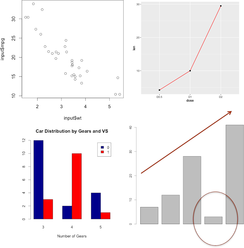
Figure 13.14: Analysis and pattern-reveal through visualization [personal file].
At this point, we will only list some simple visualization methods that are often used to reveal patterns:
scatter plots are best suited for two numeric variables;
line charts, for numeric variable and ordinal variable;
bar charts for one categorical and one numeric, or multiple categorical/nested categorical data;
boxplots, histograms, bubble charts, small multiples, etc.
An in-depth discussion of data visualization is given in Data Visualization; best practices and a more complete catalogue are provided in [83].
13.6.4 Common Statistical Procedures in R
The underlying goal of statistical analysis is to reach an understanding of the data. In this section, we show how some of the most common basic statistical concepts that can help analysts reach that goal are implemented in R; a more thorough treatment of probability and statisics notion can be found in Math & Stats Overview.
Once the data is properly organized and visual exploration has begun in earnest, the typical next step is to describe the distribution of each variable numerically, followed by an exploration of the relationships among selected variables.
The objective is to answer questions such as:
What kind of mileage are cars getting these days? Specifically, what’s the distribution of miles per gallon (mean, standard deviation, median, range, and so on) in a survey of automobile makes and models?
After a new drug trial, what is the outcome (no improvement, some improvement, marked improvement) for drug versus placebo groups? Does the gender of the participants have an impact on the outcome?
What is the correlation between income and life expectancy? Is it significantly different from zero?
Are you more likely to receive imprisonment for a crime in different regions of Canada? Are the differences between regions statistically significant?
13.6.4.1 Basic Statistics
When it comes to calculating descriptive statistics, R can basically do it all.
We start with functions that are included in the base installation. We will then look for extensions that are available through the use of user-contributed packages.
For illustrative purposes, we will use several of the variables from the Motor Trend Car Road Tests (mtcars) dataset provided in the base installation: we will focus on miles per gallon (mpg), horsepower (hp), and weight (wt):
| mpg | hp | wt | |
|---|---|---|---|
| Mazda RX4 | 21.0 | 110 | 2.620 |
| Mazda RX4 Wag | 21.0 | 110 | 2.875 |
| Datsun 710 | 22.8 | 93 | 2.320 |
| Hornet 4 Drive | 21.4 | 110 | 3.215 |
| Hornet Sportabout | 18.7 | 175 | 3.440 |
| Valiant | 18.1 | 105 | 3.460 |
Let us first take a look at descriptive statistics for all 32 models.
In the base installation, we can use the summary() function to obtain descriptive statistics.
| mpg | hp | wt | |
|---|---|---|---|
| Min. :10.40 | Min. : 52.0 | Min. :1.513 | |
| 1st Qu.:15.43 | 1st Qu.: 96.5 | 1st Qu.:2.581 | |
| Median :19.20 | Median :123.0 | Median :3.325 | |
| Mean :20.09 | Mean :146.7 | Mean :3.217 | |
| 3rd Qu.:22.80 | 3rd Qu.:180.0 | 3rd Qu.:3.610 | |
| Max. :33.90 | Max. :335.0 | Max. :5.424 |
The summary() function provides the minimum, maximum, quartiles, and mean for numerical variables, and the respective frequencies for factors and logical vectors.
In base R, the functions apply() or sapply() can be used to provide any descriptive statistics. The format in use is:
> `sapply(x, FUN, options)`where \(x\) is the data frame (or matrix) and FUN is an arbitrary function. If options are present, they’re passed to FUN.
Typical functions that can be plugged here are
mean()sd()var()min()max()median()length()range()quantile()fivenum()
The next example provides several descriptive statistics using sapply(), including the skew and the kurtosis.
mystats <- function(x, na.omit=FALSE){
                    if (na.omit)
                        x <- x[!is.na(x)]
                    m <- mean(x)
                    n <- length(x)
                    s <- sd(x)
                    skew <- sum((x-m)^3/s^3)/n
                    kurt <- sum((x-m)^4/s^4)/n - 3
                    return(c(n=n, mean=m, stdev=s,
                             skew=skew, kurtosis=kurt))
                  }

knitr::kable(sapply(mtcars[myvars], mystats))| mpg | hp | wt | |
|---|---|---|---|
| n | 32.000000 | 32.0000000 | 32.0000000 |
| mean | 20.090625 | 146.6875000 | 3.2172500 |
| stdev | 6.026948 | 68.5628685 | 0.9784574 |
| skew | 0.610655 | 0.7260237 | 0.4231465 |
| kurtosis | -0.372766 | -0.1355511 | -0.0227108 |
For cars in this sample, the mean mpg is 20.1, with a standard deviation of 6.0. The distribution is skewed to the right (\(+0.61\)) and is somewhat flatter than a normal distribution (\(-0.37\)). This is most evident if you graph the data.
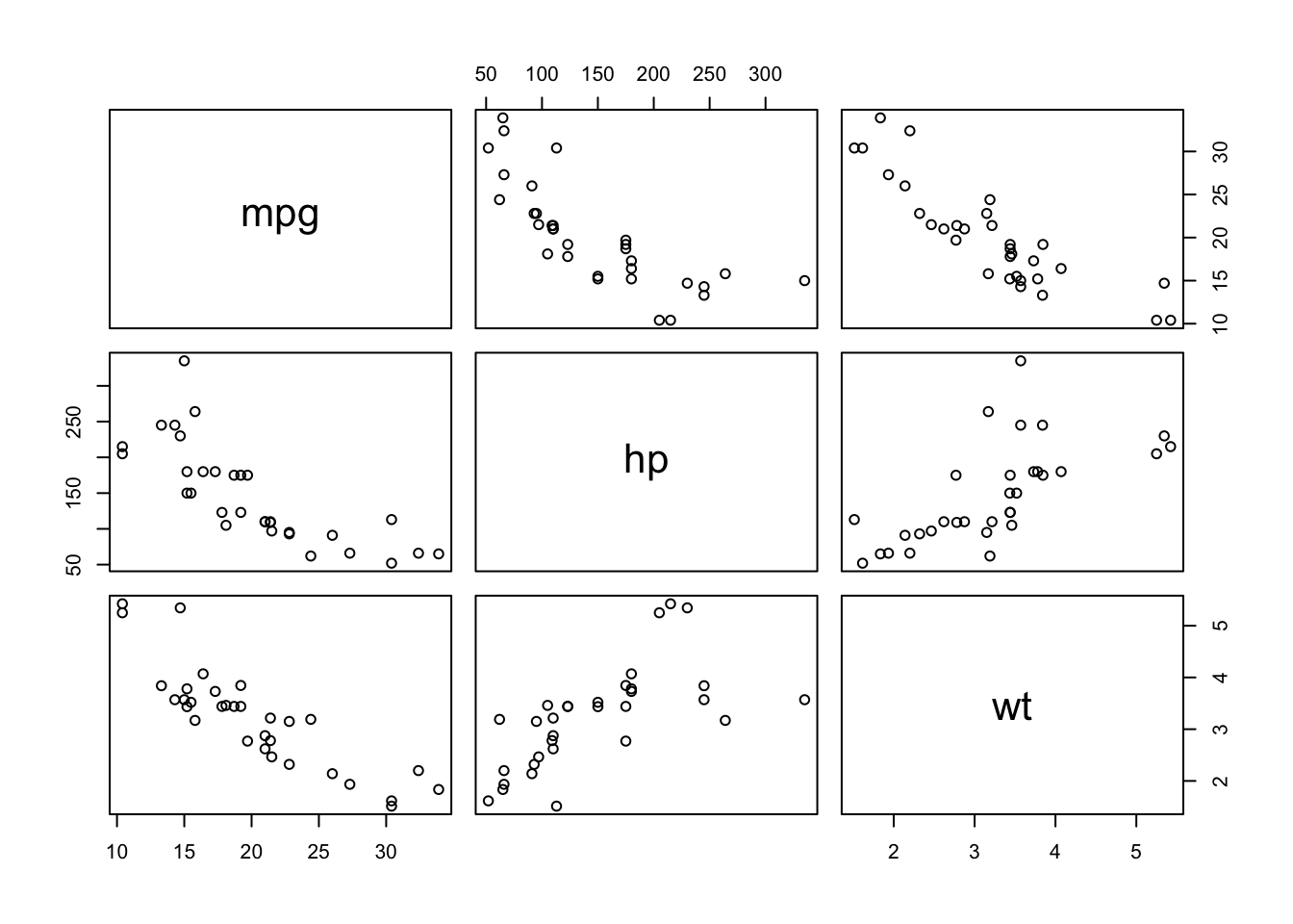
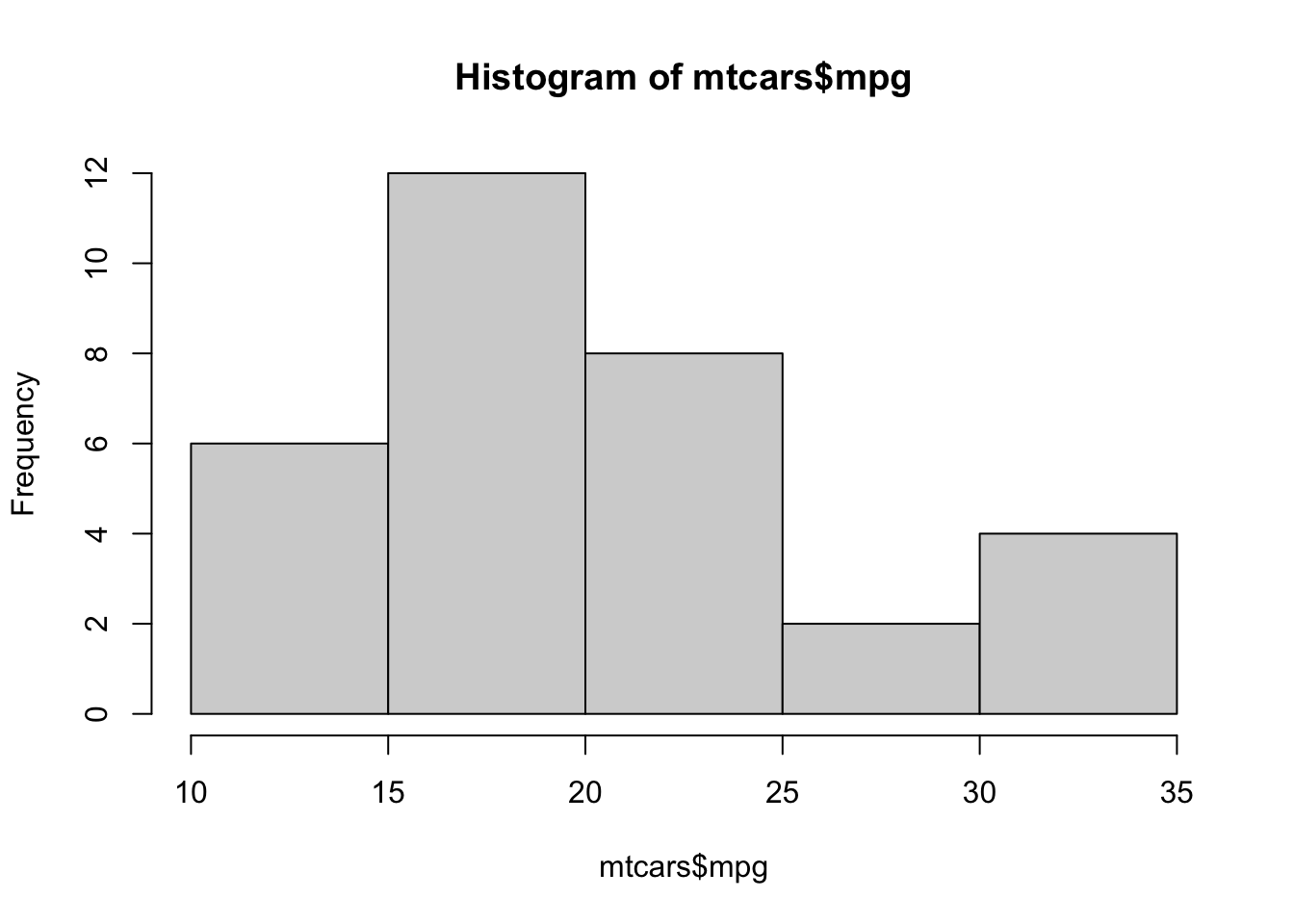
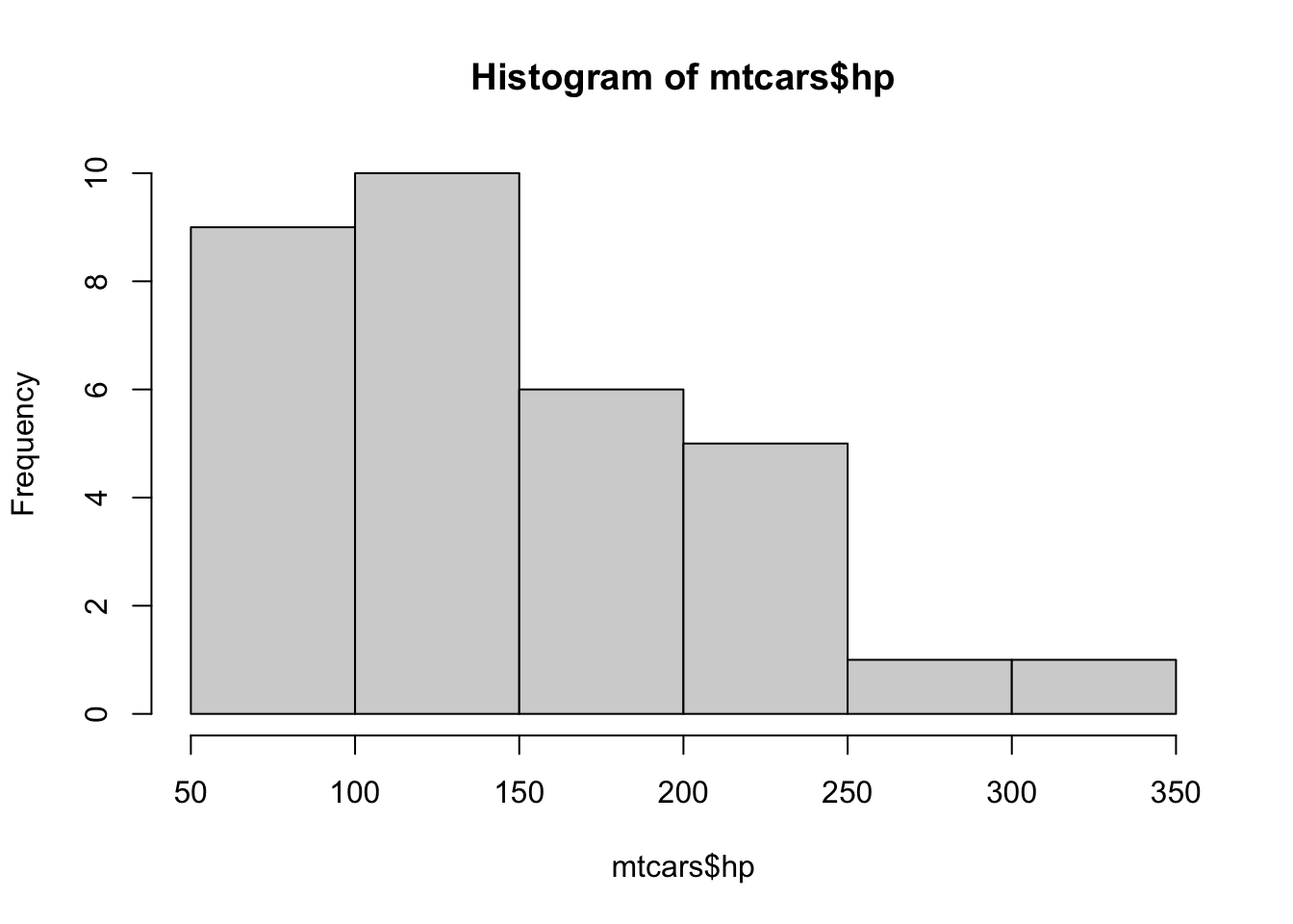
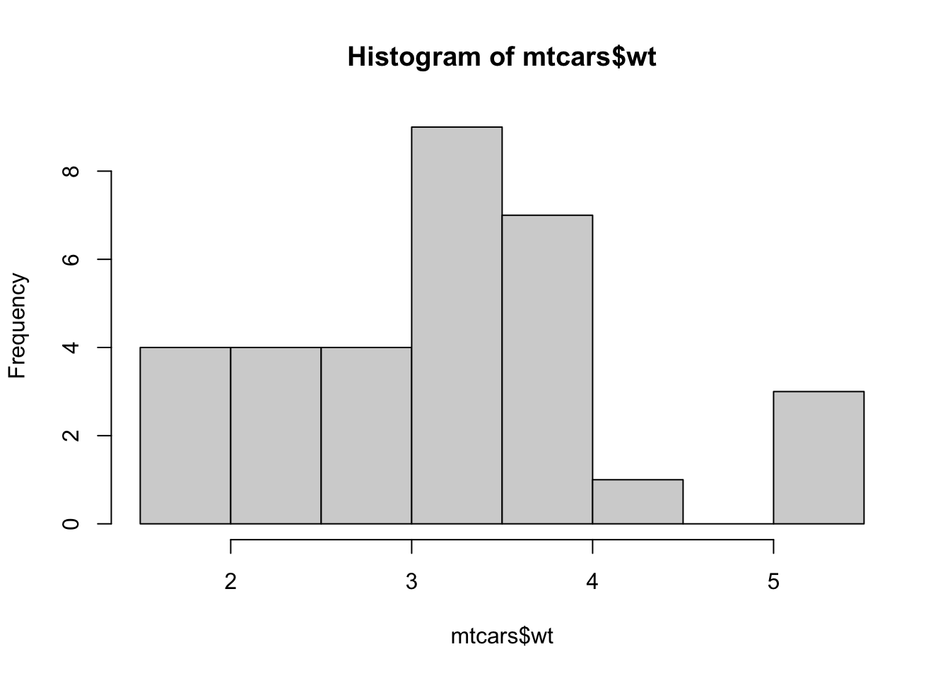
To omit missing values for the computations, we would use the option na.omit=TRUE.
# create a version of mtcars with some missing values
my.mtcars <- mtcars
my.mtcars[2,1] <- NA
my.mtcars[17,1] <- NA

knitr::kable(sapply(my.mtcars[myvars], mystats, na.omit=TRUE))| mpg | hp | wt | |
|---|---|---|---|
| n | 30.0000000 | 32.0000000 | 32.0000000 |
| mean | 20.2400000 | 146.6875000 | 3.2172500 |
| stdev | 6.1461847 | 68.5628685 | 0.9784574 |
| skew | 0.5660728 | 0.7260237 | 0.4231465 |
| kurtosis | -0.4870340 | -0.1355511 | -0.0227108 |
Notice the difference in the mpg summary.
The same table can be obtained using the dplyr functions instead.
library(dplyr)
library(e1071)
mpg = summarise(mtcars, n=n(), mean=mean(mpg),
                stdev=sd(mpg), skew=skewness(mpg), kurt=kurtosis(mpg))
hp = summarise(mtcars, n=n(), mean=mean(hp),
                stdev=sd(hp), skew=skewness(hp), kurt=kurtosis(hp))
wt = summarise(mtcars, n=n(), mean=mean(wt),
                stdev=sd(wt), skew=skewness(wt), kurt=kurtosis(wt))

pivot = t(rbind(mpg,hp,wt))
colnames(pivot) <- c("mpg","hp","wt")

knitr::kable(pivot)| mpg | hp | wt | |
|---|---|---|---|
| n | 32.000000 | 32.0000000 | 32.0000000 |
| mean | 20.090625 | 146.6875000 | 3.2172500 |
| stdev | 6.026948 | 68.5628685 | 0.9784574 |
| skew | 0.610655 | 0.7260237 | 0.4231465 |
| kurt | -0.372766 | -0.1355511 | -0.0227108 |
13.6.4.2 Hmisc and pastecs
Several packages offer functions for descriptive statistics, including Hmisc and pastecs. Because these packages are not included in the base distribution, they need to be installed on first use.
Hmisc’s describe() function returns the number of variables and observations, the number of missing and unique values, the mean, quantiles, and the five highest and lowest values.
Loading required package: latticeLoading required package: survivalLoading required package: Formula
Attaching package: 'Hmisc'The following object is masked from 'package:e1071':
imputeThe following objects are masked from 'package:dplyr':
src, summarizeThe following objects are masked from 'package:base':
format.pval, unitsmtcars[myvars]
3 Variables 32 Observations
--------------------------------------------------------------------------------
mpg
n missing distinct Info Mean Gmd .05 .10
32 0 25 0.999 20.09 6.796 12.00 14.34
.25 .50 .75 .90 .95
15.43 19.20 22.80 30.09 31.30
lowest : 10.4 13.3 14.3 14.7 15.0, highest: 26.0 27.3 30.4 32.4 33.9
--------------------------------------------------------------------------------
hp
n missing distinct Info Mean Gmd .05 .10
32 0 22 0.997 146.7 77.04 63.65 66.00
.25 .50 .75 .90 .95
96.50 123.00 180.00 243.50 253.55
lowest : 52 62 65 66 91, highest: 215 230 245 264 335
--------------------------------------------------------------------------------
wt
n missing distinct Info Mean Gmd .05 .10
32 0 29 0.999 3.217 1.089 1.736 1.956
.25 .50 .75 .90 .95
2.581 3.325 3.610 4.048 5.293
lowest : 1.513 1.615 1.835 1.935 2.140, highest: 3.845 4.070 5.250 5.345 5.424
--------------------------------------------------------------------------------The pastecs package includes the function stat.desc() that provides a
wide range of descriptive statistics:
> `stat.desc(x, basic=TRUE, desc=TRUE, norm=FALSE, p=0.95)`where \(x\) is a data frame or a time series. If basic=TRUE (the default), the number of values, null values, missing values, minimum, maximum, range, and sum are provided.
If desc=TRUE (also the default), the median, mean, standard error of the mean, 95% confidence interval for the mean, variance, standard deviation, and coefficient of variation are also provided.
Finally, if norm=TRUE (not the default), normal distribution statistics are returned, including skewness and kurtosis (with statistical significance) and the Shapiro–Wilk test of normality.
A \(p-\)value option is used to calculate the confidence interval for the mean (.95 by default).
Attaching package: 'pastecs'The following objects are masked from 'package:dplyr':
first, lastThe following object is masked from 'package:tidyr':
extract| mpg | hp | wt | |
|---|---|---|---|
| nbr.val | 32.0000000 | 32.0000000 | 32.0000000 |
| nbr.null | 0.0000000 | 0.0000000 | 0.0000000 |
| nbr.na | 0.0000000 | 0.0000000 | 0.0000000 |
| min | 10.4000000 | 52.0000000 | 1.5130000 |
| max | 33.9000000 | 335.0000000 | 5.4240000 |
| range | 23.5000000 | 283.0000000 | 3.9110000 |
| sum | 642.9000000 | 4694.0000000 | 102.9520000 |
| median | 19.2000000 | 123.0000000 | 3.3250000 |
| mean | 20.0906250 | 146.6875000 | 3.2172500 |
| SE.mean | 1.0654240 | 12.1203173 | 0.1729685 |
| CI.mean.0.95 | 2.1729465 | 24.7195501 | 0.3527715 |
| var | 36.3241028 | 4700.8669355 | 0.9573790 |
| std.dev | 6.0269481 | 68.5628685 | 0.9784574 |
| coef.var | 0.2999881 | 0.4674077 | 0.3041285 |
We will take this opportunity to caution users against relying too heavily on one (or multiple) specific packages.
13.6.4.3 Correlations
Correlation coefficients are used to describe relationships among quantitative variables. The sign \(\pm\) indicates the direction of the relationship (positive or inverse), and the magnitude indicates the strength of the relationship (ranging from 0 for no linear relationship to 1 for a perfect linear relationship).
In this section, we look at a variety of correlation coefficients, as well as tests of significance. We will use the state.x77 dataset available in the base R installation. It provides data on the population, income, illiteracy rate, life expectancy, murder rate, and high school graduation rate for the 50 US states in 1977. There are also temperature and land-area measures, but we will not be using them. In addition to the base installation, we will be using the psych and ggm packages.
R can produce a variety of correlation coefficients, including Pearson, Spearman, Kendall, partial, polychoric, and polyserial:
the Pearson product-moment coefficient assesses the degree of linear relationship between two quantitative variables;
Spearman’s rank-order coefficient assesses the degree of relationship between two rank-ordered variables;
Kendall’s tau coefficient is a nonparametric measure of rank correlation.
The cor() function produces all three correlation coefficients, whereas the cov() function provides covariances. There are many options, but a simplified format for producing correlations is
> `cor(x, use= , method= )`where \(x\) is a matrix or a data frame, and use specifies the handling
of missing data; it’s options are
all.obs(assumes no missing data);everything(any correlation involving a case with missing values will be set to missing);complete.obs(listwise deletion), andpairwise.complete.obs(pairwise deletion).
The method specifies the type of correlation; its options are pearson, spearman, and
kendall.
The default options are use ="everything" and method= "pearson".
| Population | Income | Illiteracy | Life Exp | Murder | HS Grad | |
|---|---|---|---|---|---|---|
| Population | 1.0000000 | 0.2082276 | 0.1076224 | -0.0680520 | 0.3436428 | -0.0984897 |
| Income | 0.2082276 | 1.0000000 | -0.4370752 | 0.3402553 | -0.2300776 | 0.6199323 |
| Illiteracy | 0.1076224 | -0.4370752 | 1.0000000 | -0.5884779 | 0.7029752 | -0.6571886 |
| Life Exp | -0.0680520 | 0.3402553 | -0.5884779 | 1.0000000 | -0.7808458 | 0.5822162 |
| Murder | 0.3436428 | -0.2300776 | 0.7029752 | -0.7808458 | 1.0000000 | -0.4879710 |
| HS Grad | -0.0984897 | 0.6199323 | -0.6571886 | 0.5822162 | -0.4879710 | 1.0000000 |
This produces the Pearson product-moment correlation coefficients; we can see, for example, that a strong positive correlation exists between income and HS Grad rate and that a strong negative correlation exists between Illiteracy and Life Exp.
A partial correlation is a correlation between two quantitative variables, controlling for one or more other quantitative variables; the pcor() function in the ggm package provides partial correlation coefficients (again, this package is not installed
by default, so it must be installed before first use).
The format is
> `pcor(u, S)`where \(u\) is a vector of integers, with the
first two entries representing the indices of the variables to be correlated, and
remaining numbers being the indices of the conditioning variables (that is, the variables being partialed out),
and where \(S\) is the covariance matrix among the variables.
Attaching package: 'ggm'The following object is masked from 'package:Hmisc':
rcorrcolnames(states)
pcor(c(1,5,2,3,6), cov(states))
pcor(c(1,5,2,3), cov(states))
pcor(c(1,5,2), cov(states))[1] "Population" "Income" "Illiteracy" "Life Exp" "Murder"
[6] "HS Grad"
[1] 0.3462724
[1] 0.3621683
[1] 0.4113621In this case, 0.346 is the correlation between population (variable 1) and murder rate (variable 5), controlling for the influence of income, illiteracy rate, and high school graduation rate (variables 2, 3, and 6 respectively).
The use of partial correlations is common in the social sciences.
13.6.4.4 Simple Linear Regression
In many ways, regression analysis is at the heart of statistics. It is a broad term for a set of methodologies used to predict a response variable (also called a dependent, criterion, or outcome variable) from one or more predictor variables (also called independent or explanatory variables).
In general, regression analysis can be used to
identify the explanatory variables that are related to a response variable;
describe the form of the relationships involved, and
provide an equation for predicting the response variable from the explanatory variables.
For example, an exercise physiologist might use regression analysis to develop an equation for predicting the expected number of calories a person will burn while exercising on a treadmill.
In this example, the response variable is the number of calories burned (calculated from the amount of oxygen consumed), say, and the predictor variables might include:
duration of exercise (minutes);
percentage of time spent at their target heart rate;
average speed (mph);
age (years);
gender, and
body mass index (BMI).
From a practical point of view, regression analysis would help answer questions such as:
How many calories can a 30-year-old man with a BMI of 28.7 expect to burn if he walks for 45 minutes at an average speed of 4 miles per hour and stays within his target heart rate 80% of the time?
What’s the minimum number of variables needed in order to accurately predict the number of calories a person will burn when walking?
R has powerful and comprehensive features for fitting regression models – the abundance of options can be confusing.
The basic function for fitting a linear model is lm(). The format is
> `myfit <- lm(formula, data)`where formula describes the model to be fit and data is the data frame containing the data to be used in fitting the model.
The resulting object (myfit, in this case) is a list that contains extensive information about the fitted model.
The formula is typically written as \[Y \sim X_{1}+X_{2}+\cdots+X_{k}\] where the \(\sim\) separates the response variable on the left from the predictor variables on the right, and the predictor variables are separated by \(+\) signs.
In addition to lm(), there are several functions that are useful when
generating regression models.
| Function | Action |
|---|---|
summary() |
Displays detailed results for the fitted model |
coefficients() |
Lists the model parameters (intercept and slopes) for the fitted model |
confint() |
Provides confidence intervals for the model parameters (95% by default) |
residuals() |
Lists the residual values in a fitted model |
anova() |
Generates an ANOVA table for a fitted model, or an ANOVA table comparing two or more fitted models |
plot() |
Generates diagnostic plots for evaluating the fit of a model |
predict() |
Uses a fitted model to predict response values for a new dataset |
Each of these functions is applied to the object returned by lm() in order to generate additional information based on the fitted model.
Example: the women dataset in the base installation provides the heights and
weights for a set of 15 women aged 30 to 39. Assume that we are interested in predicting the weight of an individual from her height.37
The linear regression on the data is obtained as follows:
Call:
lm(formula = weight ~ height, data = women)

Residuals:
    Min      1Q  Median      3Q     Max
-1.7333 -1.1333 -0.3833  0.7417  3.1167

Coefficients:
             Estimate Std. Error t value Pr(>|t|)
(Intercept) -87.51667    5.93694  -14.74 1.71e-09 ***
height        3.45000    0.09114   37.85 1.09e-14 ***
---
Signif. codes:  0 '***' 0.001 '**' 0.01 '*' 0.05 '.' 0.1 ' ' 1

Residual standard error: 1.525 on 13 degrees of freedom
Multiple R-squared:  0.991, Adjusted R-squared:  0.9903
F-statistic:  1433 on 1 and 13 DF,  p-value: 1.091e-14
From the output, you see that the prediction equation is \[\widehat{\text{Weight}} = -87.52 + 3.45\times \text{ Height}.\]
Because a height of 0 is impossible, there is no sense in trying to give a physical interpretation to the intercept – it merely becomes an adjustment constant (in other words, \(0\) is not in the domain of the model).
From the P(>|t|) column, we see that the regression coefficient (3.45) is significantly different from zero (\(p < 0.001\)), which indicates that there’s an expected increase of 3.45 pounds of weight for every 1 inch increase in height. The multiple R-squared coefficient (0.991) indicates that the model accounts for 99.1% of the variance in weights.
The individual weights (in pound) are:
[1] 115 117 120 123 126 129 132 135 139 142 146 150 154 159 164and their fitted values (and residuals) are
       1        2        3        4        5        6        7        8
112.5833 116.0333 119.4833 122.9333 126.3833 129.8333 133.2833 136.7333
       9       10       11       12       13       14       15
140.1833 143.6333 147.0833 150.5333 153.9833 157.4333 160.8833
          1           2           3           4           5           6
 2.41666667  0.96666667  0.51666667  0.06666667 -0.38333333 -0.83333333
          7           8           9          10          11          12
-1.28333333 -1.73333333 -1.18333333 -1.63333333 -1.08333333 -0.53333333
         13          14          15
0.01666667 1.56666667 3.11666667 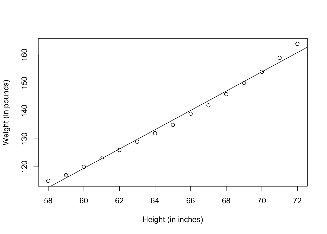
13.6.4.5 Bootstrapping
Bootstrapping is a powerful and elegant approach to estimating the sampling distribution of specific statistics. It can be implemented in many situations where asymptotic results are difficult to find or otherwise unsatisfactory.
Bootstrapping proceeds using three steps:
resample the dataset (with replacement) many times over (typically on the order of 10,000);
calculate the desired statistic from each resampled dataset;
use the distribution of the resampled statistics to estimate the standard error of the statistic (normal approximation method) or construct a confidence interval using quantiles of that distribution (percentile method).
There are several ways to bootstrap in R. As an example, say that we want to estimate the standard error and 95% confidence interval for the coefficient of variation (CV), defined as \(\sigma/\mu\), for a random variable \(X\).
We will illustrate the procedure with generated values of \(X\sim \mathcal{N}(1,1)\):
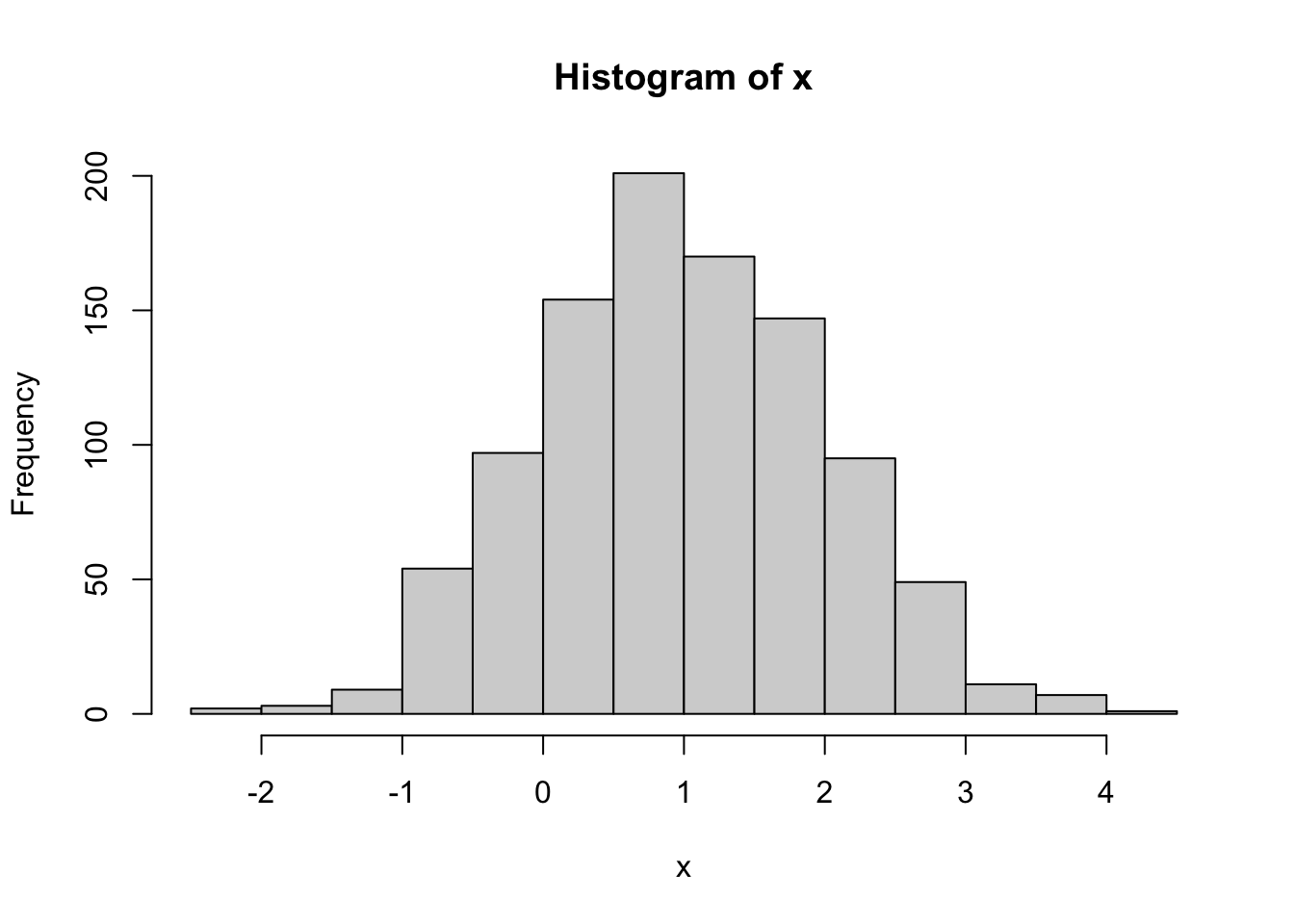
[1] 1.014057The user must provide code to calculate the statistic of interest as a function.
The replicate() function is the base R tool for repeating function calls. Within that function, we nest a call to covfun() and a call to sample the data with replacement using the sample() function.
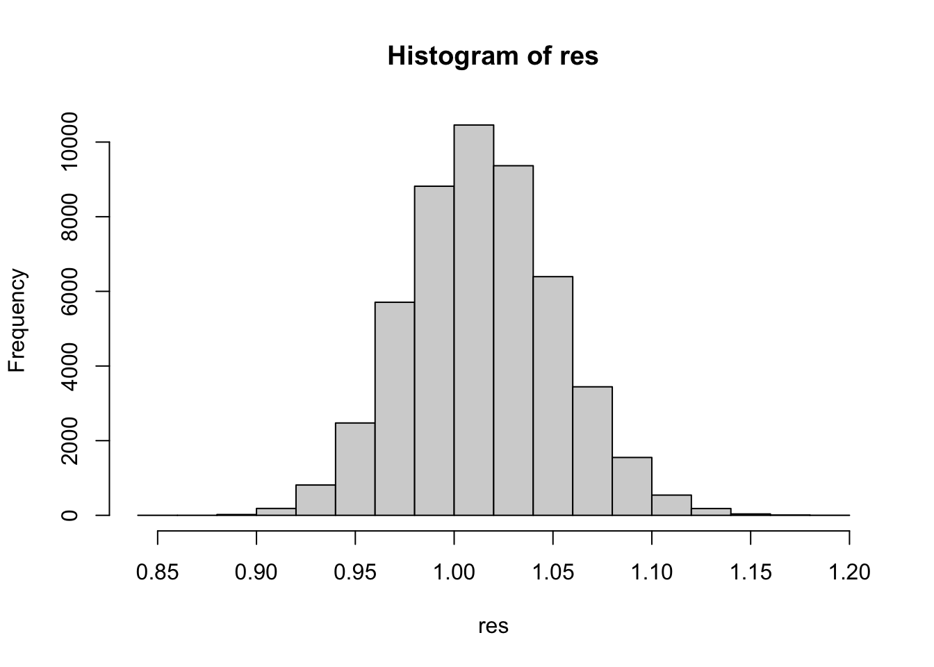
     2.5%     97.5%
0.9432266 1.0917185
This seems reasonable, as we would expect the CVs to be centered around 1.
The percentile interval is easy to calculate from the observed bootstrapped statistics. If the distribution of the bootstrap samples is approximately normally distributed, a \(t\) interval could be created bycalculating the standard deviation of the bootstrap samples and finding the appropriate multiplier for the confidence interval. Plotting the bootstrap sample estimates is helpful to determine the form of the bootstrap distribution.
The framework can also be extended to include non-linear models, correlated variables, probability estimation, and/or multivariate models; any book on statistical analysis contains at least one chapter or two on the topic (see [11], [84], for instance).
We will not pursue the topic further except to say that regression analysis is one of the arrows that every data scientist should have in their quiver.
13.6.5 Quantitative Methods
We provided a list of quantitative methods in Data Collection, Storage, Processing, and Modeling; we finish this section by expanding on a few of them. More details
13.6.5.1 Classification and Supervised Learning Tasks
Classification is one of the cornerstones of machine learning. Instead of trying to predict the numerical value of a response variable (as in regression), a classifier uses historical data[This training data usually consists of a randomly selected subset of the labeled (response) data.] to identify general patterns that could lead to observations belonging to one of several pre-defined categories.
For instance, if a car insurance company only has resources to investigate up to 20% of all filed claims, it could be useful for them to predict:
whether a claim is likely to be fraudulent;
whether a customer is likely to commit fraud in the near future;
whether an application for a policy is likely to result in a fraudulent claim;
the amount by which a claim will be reduced if it is fraudulent, etc.
Analysts and machine learning practitioners use a variety of different techniques to carry this process out (see Figure 13.15 for an illustration, and Machine Learning 101 and [85]–[87], in general, for more details), but the general steps always remain the same:
use training data to teach the classifier;
test/validate the classifier using hold-out data;
if it passes the test, use the classifier to classify novel instances.

Figure 13.15: The trousers of classification [personal file].
Some classifiers (such as deep learning neural nets) are ‘black boxes’: they might be very good at classification, but they are not explainable.
In some instances, that is an acceptable side effect of the process, in others, it might not be – if an individual is refused refugee status, say, they might rightly want to know why.
13.6.5.2 Unsupervised Learning Techniques
The hope of artificial intelligence is that intelligent behaviours will eventually be able to be automated. For the time being, however, that is still very much a work in progress.
But one of the challenges in that process is that not every intelligent behaviour arises from a supervised process.
Classification, for instance, is the prototypical supervised task: can we learn from historical/training examples? It seems like a decent approach to learning: evidence should drive the process.
But there are limitations to such an approach: it is difficult to make a conceptual leap solely on the basis of training data,[If our teaching experience is anything to go by…] if only because the training data data might not be representative of the system, or because the learner target task is too narrow.
In unsupervised learning, we learn without examples, based solely on what is found in the data. There is no specific question to answer (in the classification sense), other than: what can we learn from the data?
Typical unsupervised learning tasks include:
clustering (novel categories);
association rules mining;
recommender systems, etc.
For instance, an online bookstore might want to make recommendations to customers concerning additional items to browse (and hopefully purchase) based on their buying patterns in prior transactions, the similarity between books, and the similarity between customer segments:
But what are those patterns?
How do we measure similarity?
What are the customer segments?
Can any of that information be used to create promotional bundles?
The lack of a specific target makes unsupervised learning much more difficult than supervised learning, as does the challenges of validating the results. This contributes to the proliferation of clustering algorithms and cluster quality metrics.
More general information and details on clutering can be found in Machine Learning 101 and in [76], [87], [88].
13.6.5.3 Other Machine Learning Tasks
These scratch but a miniscule part part of the machine learning ecosystem. Other common tasks include [77]:
profiling and behaviour description;
link prediction;
data reduction;
influence/causal modeling, etc.
to say nothing of more sophisticated learning frameworks (semi-supervised, reinforcement [89], deep learning [90], etc.).
13.6.5.4 Time Series Analysis and Process Monitoring
Processes are often subject to variability:
variability due the cumulative effect of many small, essentially unavoidable causes (a process that only operates with such common causes is said to be in (statistical) control;
variability due to special causes, such as improperly adjusted machines, poorly trained operators, defective materials, etc. (the variability is typically much larger for special causes, and such processes are said to be out of (statistical) control.
The aim of statistical process monitoring (SPM) is to identify occurrence of special causes. This is often done via time series analysis.
Consider \(n\) observations \(\{x_1,\ldots,x_n\}\) arising from some collection of processes. In practice, the index \(i\) is often a time index or a location index, i.e., the \(x_i\) are observed in sequence or in regions.38
The processes that generate the observations could change from one time/location to the next due to:
external factors (war, pandemic, regime change, election results, etc.), or
internal factors (policy changes, modification of manufacturing process, etc.).
In such caes, the mean and standard deviation alone might not provide a useful summary of the situation.
To get a sense of what is going on with the data (and the associated system), it could prove preferable to plot the data in the order that it has been collected (or according to geographical regions, or both).
The horizontal coordinate would then represent:
the time of collection \(t\) (order, day, week, quarter, year, etc.), or
the location \(i\) (country, province, city, branch, etc.).
The vertical coordinate represents the observations of interest \(x_t\) or \(x_i\) (see Figure @ for an example).
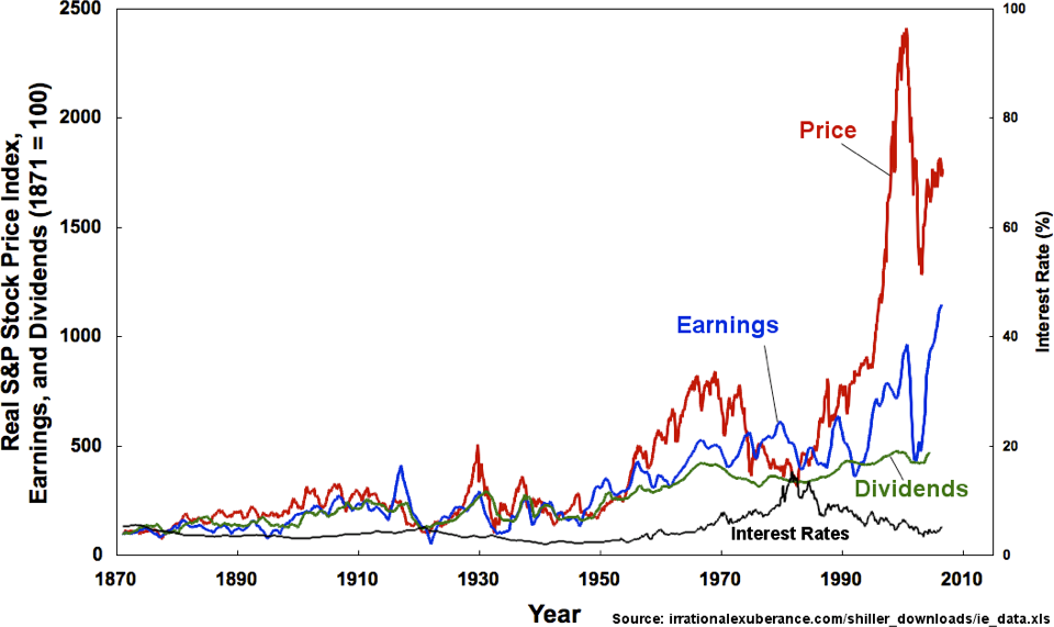
Figure 13.16: Real S&P stock price index (red), earnings (blue), and dividends (green), together with interest rates (black), from 1871 to 2009 [R.J. Shiller].
In process monitoring terms, we may be able to identify potential special causes by identifying trend breaks, cycles discontinuities, or level shifts in time series.
For instance, consider the three time series of Figure 13.17.
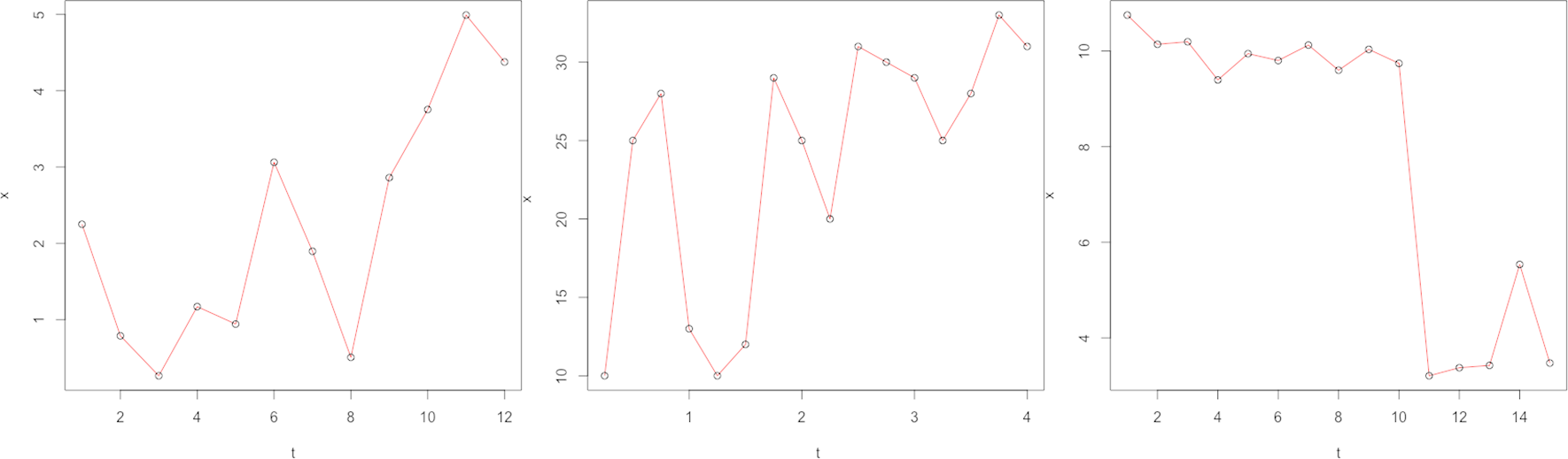
Figure 13.17: Sales (in 10,000’s$) for 3 different products – years (left), quarters (middle), weeks (right) [personal file].
Is any action required?
in the first example (left), there are occasional drops in sales from one year to the next, but the upward trend is clear – we see the importance of considering the full time series; if only the last two points are presented to stockholders, say, they might conclude that action is needed, whereas the whole series paints a more positive outlook;
in the second case (middle), there is a cyclic effect with increases from Q1 to Q2 and from Q2 to Q3, but decreases from Q3 to Q4 and from Q4 to Q1. Overall, we also see an upward trend – the presence of regular patterns is a positive development;
finally, in the last example (right), something clearly happened after the tenth week, causing a trend level shift. Whether it is due to internal or external factors depends on the context, which we do not have at our disposal, but some action certainly seems to be needed.
We might also be interested in using historical data to forecast the future behaviour of the variable. This is similar to the familiar analysis goals of:
finding patterns in the data, and
creating a (mathematical) model that captures the essence of these patterns.
Time series patterns can be quite complex and must often be broken down into multiple component models (trend, seasonal, irregular, etc.).
Typically, this can be achieved with fancy analysis methods, but it is not a simple topic, in general. Thankfully, there are software libraries that can help.
13.6.5.5 Anomaly Detection
The special points from process monitoring are anomalous in the sense that something unexpected happens there, something that changes the nature of the data pre- and post-break.
In a more general context, anomalous observations are those that are atypical or unlikely.
From an analytical perspective, anomaly detection can be approached using supervised, unsupervised, or conventional statistical methods.
The discipline is rich and vibrant (and the search for anomalies can end up being an arms race against the “bad guys”), but it is definitely one for which analysts should heed contextual understanding – blind analysis leads to blind alleys! A more thorough treatment is provided in [91].
There is a lot more to say on the topic of data analysis – we will delve into various topics in detail in subsequent modules.
In what follows, we will spend some time discussing the preparation of data for analysis.
References
[11] R. V. Hogg and E. A. Tanis, Probability and statistical inference, 7th ed. Pearson/Prentice Hall, 2006.
[12] T. H. Davenport and D. J. Patil, “Data scientist: The sexiest job of the 21st century,” Harvard Business Review, Oct. 2012,Available: https://hbr.org/2012/10/data-scientist-the-sexiest-job-of-the-21st-century
[13] L. Donnelly, “Robots are better than doctors at diagnosing some cancers, major study finds,” The Telegraph, May 2018.
[14] P. A. B. Bien Nicholas AND Rajpurkar, “Deep-learning-assisted diagnosis for knee magnetic resonance imaging: Development and retrospective validation of mrnet,” PLOS Medicine, vol. 15, no. 11, pp. 1–19, 2018, doi: 10.1371/journal.pmed.1002699.
[15] BeauHD, “Google ai claims 99 percent accuracy in metastatic breast cancer detection,” Slashdot.com, Oct. 2018.
[16] Columbia University Irving Medical Center, “Data scientists find connections between birth month and health,” Newswire.com, Jun. 2015.
[17] “Scientists using gps tracking on endangered dhole wild dogs.” Live View GPS, Oct. 2018.
[18] S. Reichman, “These ai-invented paint color names are so bad, they’re good,” Curbed, May 2017.
[19] K. Hao, “We tried teaching an ai to write christmas movie plots. Hilarity ensued. Eventually,” MIT Technology Review, Dec. 2018.
[20] E. Betuel, “Math model determines who wrote beatles’ "in my life": Lennon or mccartney?” Inverse, Jul. 2018.
[21] Indiana University, “Scientists use instagram data to forecast top models at new york fashion week,” Science Daily, Sep. 2015.
[22] J. Hiner, “How big data will solve your email problem,” ZDNet, Oct. 2013.
[23] B. Smith, “Artificial intelligence better than physicists at designing quantum science experiments,” ABC Science, Oct. 2018.
[24] A. Van Dam, “This researcher studied 400,000 knitters and discovered what turns a hobby into a business,” Washington Post, Nov. 2018.
[25] E. Yong, “Wait, have we really wiped out 60% of animals?” The Atlantic, Oct. 2018.
[26] J. Dastin, “Amazon scraps secret ai recruiting tool that showed bias against women,” Reuters, Oct. 2018.
[27] “Facebook documents seized by mps investigating privacy breach.” BBC News, Nov. 2018.
[28] D. Wakabayashi, “Firm led by google veterans uses a.i. To ‘nudge’ workers toward happiness,” New York Times, Dec. 2018.
[29] S. Ramachandran and J. Flint, “At netflix, who wins when it’s hollywood vs.the algorithm?” Wall Street Journal, Nov. 2018.
[30] M. Jing, “AlphaGo vanquishes world’s top go player, marking a.i.’s superiority over human mind,” South China Morning Post, May 2017.
[31] D. Lewis, “An ai-written novella almost won a literary prize,” Smithsonian Magazine, Mar. 2016.
[32] E. Mack, “Elon musk: Artificial intelligence may spark world war iii,” CNET, Sep. 2017.
[33] T. Rikert, “A.I. Hype has peaked so what’s next?” TechCrunch, Sep. 2017.
[34] J. C. Scott, Against the grain: A deep history of the earliest states. New Haven: Yale University Press, 2017.
[35] R. Mérou, “Conceptual map of free software.” Wikimedia, 2010.
[36] Henning (WMDE), “UML diagram of the wikibase data model.” Wikimedia.
[37] Wooptoo, “Entity - relationship model.” Wikimedia.
.png)
[38] S. L. Lee and D. Baer, “20 cognitive biases that screw up your decisions,” Business Insider, Dec. 2015.
[39] “Cognitive biases.” The Decision Lab.
[40] R. Schutt and C. O’Neill, Doing data science: Straight talk from the front line. O’Reilly, 2013.
[41] “Research integrity & ethics.” Memorial University of Newfoundland.
[42] “A conversation with julie paquette: Ethics in quantitative contexts.” Paquette, J. and Boily, P.
[43] “Code of ethics/conducts.” Certified Analytics Professional.
[45] “ACM code of ethics and professional conduct.” Association for Computing Machinery.
[46] K. Fung, “The ethics conversation we’re not having about data,” Harvard Business Review, Nov. 2015.
[47] C. O’Neil, Weapons of math destruction: How big data increases inequality and threatens democracy. Crown, 2016.
[48] M. Chen, “Is ‘big data’ actually reinforcing social inequalities?” The Nation, Sep. 2013.
[49] R. W. Paul and L. Elder, Understanding the foundations of ethical reasoning, 2nd ed. Foundation for Critical Thinking, 2006.
[50] “Centre for big data ethics, law, and policy.” Data Science Institute, University of Virginia.
[51] “Open data.” Wikipedia.
[52] D. Brin, The transparent society: Will technology force us to choose between privacy and freedom? Perseus, 1998.
[53] “Open up guide: Using open data to combat corruption.” Open Data Charter, 2017.
[54] J. S. A. Corey, The Expanse. Orbit Books.
[55] N. Cohn, “How one 19-year-old illinois man is distorting national polling averages,” The Upshot, 2016.
[56] A. Gumbus and F. Grodzinsky, “Era of big data: Danger of descrimination,” ACM SIGCAS Computers and Society, vol. 45, no. 3, pp. 118–125, 2015.
[58] M. Judge, “Facial-recognition technology affects african americans more often,” The Root, 2016.
[59] I. Asimov, Foundation series. Gnome Press, Spectra, Doubleday.
[60] I. Stewart, “The fourth law of humanics,” Nature, vol. 535, 2016.
[61] J. Cranshaw, R. Schwartz, J. I. Hong, and N. M. Sadeh, “The livehoods project: Utilizing social media to understand the dynamics of a city,” in ICWSM, 2012.Available: http://dblp.uni-trier.de/db/conf/icwsm/icwsm2012.html#CranshawSHS12
[68] S. E. Brossette, A. P. Sprague, J. M. Hardin, K. B. Waites, W. T. Jones, and S. A. Moser, “Association Rules and Data Mining in Hospital Infection Control and Public Health Surveillance,” Journal of the American Medical Informatics Association, vol. 5, no. 4, pp. 373–381, Jul. 1998, doi: 10.1136/jamia.1998.0050373.
[69] M. Kosinski and Y. Wang, “Deep neural networks are more accurate than humans at detecting sexual orientation from facial images,” Journal of Personality and Social Psychology, vol. 114, no. 2, pp. 246–257, Feb. 2018.
[70] J. Taylor, “Four problems in using crisp-dm and how to fix them,” KDnuggets.com, 2017.
[71] P. Boily, “Non-technical aspects of consulting,” Introduction to Quantitative Consulting, 2021.
[72] P. Boily, Introduction to Quantitative Consulting, 2021.
[73] A. De Mauro, M. Greco, and M. Grimaldi, “A formal definition of big data based on its essential features,” Library Review, vol. 65, no. 3, pp. 122–135, 2016.
[74] D. Robinson, “What’s the difference between data science, machine learning, and artificial intelligence?” Variance Explained, Jan. 2018,Available: http://varianceexplained.org/r/ds-ml-ai/
[75] D. Woods, “Bitly’s hilary mason on "what is a data scientist?",” Forbes, Mar. 2012,Available: https://www.forbes.com/sites/danwoods/2012/03/08/hilary-mason-what-is-a-data-scientist/#1189ca465502
[76] C. C. Aggarwal and C. K. Reddy, Eds., Data clustering: Algorithms and applications. CRC Press, 2014.Available: http://www.charuaggarwal.net/clusterbook.pdf
[77] F. Provost and T. Fawcett, Data science for business. O’Reilly, 2015.
[78] A. M. Masci et al., “An improved ontological representation of dendritic cells as a paradigm for all cell types,” BMC Bioinformatics, 2009.
[79] boot4life, “What json structure to use for key-value pairs.” StackOverflow, Jun. 2016.
[80] V. M. Chawla, ERD "Crow’s Foot" Relationship Symbols Cheat Sheet, 2013.
[81] N. Feldman, Data Lake or Data Swamp?, 2015.
[82] P. Hapala et al., “Mapping the electrostatic force field of single molecules from high-resolution scanning probe images,” Nature Communications, vol. 7, no. 11560, 2016.
[83] P. Boily, S. Davies, and J. Schellinck, Practical data visualization. Data Action Lab/Quadrangle, 2021.
[84] P. Boily, MAT2377 - Probability and Statistics for Engineers.
[85] T. Hastie, R. Tibshirani, and J. Friedman, The elements of statistical learning: Data mining, inference, and prediction, 2nd ed. Springer, 2008.
[87] C. C. Aggarwal, Data mining: The textbook. Cham: Springer, 2015. doi: 10.1007/978-3-319-14142-8.
[88] Wikipedia, “Cluster analysis algorithms.”
[89] R. Sutton and G. Barto, Reinforcement learning: An introduction. MIT Press, 2018.
[90] I. Goodfellow, Y. Bengio, and A. Courville, Deep learning. MIT press Cambridge, 2016.
[91] Y. Cissokho, S. Fadel, R. Millson, R. Pourhasan, and P. Boily, “Anomaly Detection and Outlier Analysis,” Data Science Report Series, 2020.
In practice, more complex databases are used.↩︎
Or ‘On’ and ‘Off’, ‘TRUE’ and ‘FALSE’.↩︎
Note that it also happens with small, well-organized, and easily contained projects. It happens all the time, basically.↩︎
“Every model is wrong; some models are useful.” George Box.↩︎
We are obviously not implying that these individuals have no ethical principles or are unethical; rather, that the opportunity to establish what these principles might be, in relation with their research, may never have presented itself.↩︎
This is not to say that ethical issues have miraculously disappeared – Volkswagen, Whole Foods Markets, General Motors, Cambridge Analytica, and Ashley Madison, to name but a few of the big data science and data analysis players, have all recently been implicated in ethical lapses [46]. More dubious examples can be found in [47], [48].↩︎
Truth be told, choosing wisely is probably the the most difficult aspect of a data science project.↩︎
How long does it take Netflix to figure out that you no longer like action movies and want to watch comedies instead, say? How long does it take Facebook to recognize that you and your spouse have separated and that you do not wish to see old pictures of them in your feed?↩︎
Many newly-minted data scientists have not had enough experience with effective team work, and they are likely to underestimate the challenges that usually arise from such an endeavour.↩︎
Note that individuals can play more than one role on a team.↩︎
They may also need to shield the team from clients/stakeholders.↩︎
Questions can also be asked in an unsupervised manner, see [76], [77], among others, and Quantitative Methods (#DBSFPIgifd-qm), briefly.↩︎
Unless we’re talking about quantum physics and then all bets are off – nobody has the slightest idea why things happen the way they do, down there.↩︎
According to the adage, “data is not information, information is not knowledge, knowledge is not understanding, understanding is not wisdom.” (C.Stoll, attributed).↩︎
We could facetiously describe ontologies as “data models on steroids.”↩︎
“Times change, and we change with them.” C.Huberinus↩︎
What does that make the other components?↩︎
A similar approach underlies most of modern text mining, natural language processing, and categorical anomaly detection. Information usually gets lost in the process, which explains why meaningful categorical analyses tend to stay fairly simple.↩︎
An equation to predicting weight from height could help identifying individuals who are possibly overweight (or underweight), say.↩︎
In the first situation, the observations form a time series.↩︎