Module 5 Overview of Probability Theory
Data analysis is sometimes presented in a ``point-and-click manner,’’ with tutorials often bypassing foundations in probability and statistics to focus on software use and specific datasets. While modern analysts do not always need to fully understand the theory underpinning the methods that they use, understanding some of the basic concepts can only lead to long-term benefits. In this module, we introduce some of the crucial probabilistic notions that will help analysts get the most out of their data.
5.1 Basics
Probability theory is the mathematical discipline relating to the numerical description of the likelihood of an event.
5.1.1 Sample Spaces and Events
Throughout, we will deal with random experiments (e.g., measurements of speed/ weight, number and duration of phone calls, etc.).
For any “experiment,” the sample space is defined as the set of all its possible outcomes, often denoted by the symbol \({\cal S}\). A sample space can be discrete or continuous. An event is a collection of outcomes from the sample space \({\cal S}\). Events will be denoted by \(A\), \(B\), \(E_1\), \(E_2\), etc.
Toss a fair coin – the corresponding (discrete) sample space is \({\cal S} =\{\mbox{Head, Tail}\}\).
Roll a die – the corresponding (discrete) sample space is \({\cal S}=\left\{ 1,2,3,4,5,6 \right\}\), with various events represented by
rolling an even number: \(\left\{ 2,4,6 \right\}\);
rolling a prime number: \(\left\{ 2,3,5 \right\}\).
Suppose we measure the weight (in grams) of a chemical sample – the (continuous) sample space can be represented by \(\mathcal{S}=(0,\infty)\), the positive half line, and various events by subsets of \(\mathcal{S}\), such as
sample is less than 1.5 grams: \((0,1.5)\);
sample exceeds 5 grams: \((5,\infty)\).
For any events \(A,B\subseteq {\cal S}\):
the union \(A\cup B\) of \(A\) and \(B\) are all outcomes in \({\cal S}\) contained in either \(A\) or \(B\);
the intersection \(A\cap B\) of \(A\) and \(B\) are all outcomes in \({\cal S}\) contained in both \(A\) and \(B\);
the complement \(A^c\) of \(A\) (sometimes denoted \(\overline{A}\) or \(-A\)) is the set of all outcomes in \({\cal S}\) that are not in \(A\).
If \(A\) and \(B\) have no outcomes in common, they are mutually exclusive; which is denoted by \(A\cap B=\text{Var}nothing\) (the empty set). In particular, \(A\) and \(A^{c}\) are always mutually exclusive.2
Roll a die and let \(A=\left\{ 2,3,5 \right\}\) (a prime number) and \(B=\left\{ 3,6 \right\}\) (multiples of \(3\)). Then \(A\cup B=\left\{ 2,3,5,6 \right\}\), \(A\cap B=\left\{3 \right\}\) and \(A^{c}=\left\{ 1,4,6 \right\}\).
\(100\) plastic samples are analyzed for scratch and shock resistance.
shock resistance high low scratch high \({70}\) \(4\) resistance low \(1\) \(25\) If \(A\) is the event that a sample has high shock resistance and \(B\) is the event that a sample has high scratch residence, then \(A\cap B\) consists of \(70\) samples.
5.1.2 Counting Techniques
A two-stage procedure can be modeled as having \(k\) bags, with \(m_1\) items in the first bag, …, \(m_k\) items in \(k\)-th bag.
The first stage consists of picking a bag, and the second stage consists of drawing an item out of that bag. This is equivalent to picking one of the \(m_1+\cdots+m_k\) total items.
If all the bags have the same number of items \[m_1=\cdots=m_k=n,\] then there are \(kn\) items in total, and this is the total number of ways the two-stage procedure can occur.
How many ways are there to first roll a die and then draw a card from a (shuffled) \(52-\)card pack?
Answer: there are \(6\) ways the first step can turn out, and for each of these (the stages are independent, in fact) there are \(52\) ways to draw the card. Thus there are \(6\times52=312\) ways this can turn out.
How many ways are there to draw two tickets numbered \(1\) to \(100\) from a bag, the first with the right hand and the second with the left hand?
Answer: There are \(100\) ways to pick the first number; for each of these there are \(99\) ways to pick the second number. Thus \(100\times 99=9900\) ways.
Multi-Stage Procedures
A \(k\)-stage process is a process for which:
there are \(n_1\) possibilities at stage 1;
regardless of the 1st outcome there are \(n_2\) possibilities at stage 2,
…
regardless of the previous outcomes, there are \(n_k\) choices at stage \(k\).
There are then \[n_1 \times n_2\cdots\times n_k\] total ways the process can turn out.
5.1.3 Ordered Samples
Suppose we have a bag of \(n\) billiard balls numbered \(1,\ldots,n\). We can draw an ** ordered sample** of size \(r\) by picking balls from the bag:
with replacement, or
without replacement.
With how many different collection of \(r\) balls can we end up in each of those cases (each is an \(r\)-stage procedure)?
Key Notion: all the object (balls) can be differentiated (using numbers, colours, etc.)
Sampling With Replacement (Order Important)
If we replace each ball into the bag after it is picked, then every draw is the same (there are \(n\) ways it can turn out).
According to our earlier result, there are \[\underbrace{\ n\times n \times \cdots \times n\ }_{\text{$r$ stages}}= n^r\] ways to select an ordered sample of size \(r\) with replacement from a set with \(n\) objects \(\left\{ 1,2,\ldots,n \right\}\).
Sampling Without Replacement (Order Important)
If we do not replace each ball into the bag after it is drawn, then the choices for the second draw depend on the result of the first draw, and there are only \(n-1\) possible outcomes.
Whatever the first two draws were, there are \(n-2\) ways to draw the third ball, and so on.
Thus there are \[\underbrace{n\times (n-1)\times\cdots\times (n-r+1)}_{\text{$r$ stages}} = {_nP_r}\ \ \text{ (common symbol)}\] ways to select an ordered sample of size \(r\le n\) without replacement from a set of \(n\) objects \(\left\{ 1,2,\ldots,n \right\}\).
Factorial Notation
For a positive integer \(n\), write \[n!=n(n-1)(n-2)\cdots1.\] There are two possibilities:
when \(r=n\), \(_nP_r=n!\), and the ordered selection (without replacement) is called a permutation;
when \(r<n\), we can write \[\begin{aligned} _nP_r&= \frac{n(n-1)\cdots(n-r+1)}{} \frac {(n-r)\cdots 1} {(n-r)\cdots 1} \\&= \frac{n!}{(n-r)!}=n\times \cdots \times (n-r+1).\end{aligned}\]
By convention, we set \(0!=1\), so that \[_nP_r=\frac{n!}{(n-r)!},\quad \text{for all $r\le n$.}\]
In how many different ways can 6 balls be drawn in order without replacement from a bag of balls numbered 1 to 49?
Answer: We compute \[_{49}P_6=49\times 48\times 47\times 46\times 45\times 44 = 10,068,347,520.\] This is the number of ways the actual drawing of the balls can occur for Lotto 6/49 in real-time (balls drawn one by one).
How many 6-digits PIN codes can you create from the set of digits \(\{0,1,\ldots,9\}\)?
Answer: If the digits may be repeated, we see that \[10\times 10\times 10\times 10\times 10\times 10=10^6=1,000,000.\] If the digits may not be repeated, we have instead \[_{10}P_6=10\times 9\times 8\times 7\times 6\times 5=151,200.\]
5.1.4 Unordered Samples
Suppose now that we cannot distinguish between different ordered samples; when we look up the Lotto 6/49 results in the newspaper, for instance, we have no way of knowing the order in which the balls were drawn: \[1-2-3-4-5-6\] could mean that the first drawn ball was ball # \(1\), the second drawn ball was ball # \(2\), etc., but it could also mean that the first ball drawn was ball # \(4\), the second one, ball # \(3\), etc., or any other combinations of the first 6 balls.
Denote the (as yet unknown) number of unordered samples of size \(r\) from a set of size \(n\) by \(_nC_r\). We can derive the expression for \(_nC_r\) by noting that the following two processes are equivalent:
take an ordered sample of size \(r\) (there are \(_nP_r\) ways to do this);
take an unordered sample of size \(r\) (there are \(_nC_r\) ways to do this) and then rearrange (permute) the objects in the sample (there are \(r!\) ways to do this).
Thus \[\begin{aligned} _nP_r = {_nC_r}\times r!&\implies& _nC_r = \frac{ _nP_r} {r!} = \frac{n!}{(n-r)!\ r!} = \binom n r\,.\end{aligned}\] This last notation is called a binomial coefficient (read as “\(n\)-choose-\(r\)”) and is commonly used in textbooks.
in how many ways can the “Lotto 6/49 draw” be reported in the newspaper (where they are always reported in increasing order)?
Answer: this number is the same as the number of unordered samples of size 6 (different re-orderings of same 6 numbers are indistinguishable), so \[\begin{aligned} _{49}C_6&=\binom {49}6 =\frac{49\times 48\times 47\times 46\times 45\times 44} {6\times 5\times4\times3\times2\times 1} \\ &= \frac{ 10,068,347,520 }{720} = 13,983,816\,.\end{aligned}\] There exists a variety of binomial coefficient identities, such as \[\begin{aligned} \binom{n}{k}&=\binom{n}{n-k},\quad \text{for all $0\leq k\leq n$}, \\ \sum_{k=0}^n\binom{n}{k}&=2^n, \quad \text{for all $0\leq n$}, \\ \binom{n+1}{k+1}&=\binom{n}{k}+\binom{n}{k+1},\quad \text{for all $0\leq k\leq n-1$} \\ \sum_{j=k}^n\binom{j}{k}&=\binom{n+1}{k+1}, \quad \text{for all $0\leq n$, etc.}.\end{aligned}\]
5.1.5 Probability of an Event
For situations where we have a random experiment which has exactly \(N\) possible mutually exclusive, equally likely outcomes, we can assign a probability to an event \(A\) by counting the number of outcomes that correspond to \(A\) – its relative frequency.
If that count is \(a\), then \[P(A) = \frac{a}{N}.\] The probability of each individual outcome is thus \(1/N\).
Toss a fair coin – the sample space is \({\cal S} = \{\mbox{Head, Tail}\}\), i.e., \(N=2\). The probability of observing a Head on a toss is thus \(\frac{1}{2}.\)
Throw a fair six sided die. There are \(N=6\) possible outcomes. The sample space is \[{\cal S} = \{1,2,3,4,5,6\}.\] If \(A\) corresponds to observing a multiple of \(3\), then \(A=\{3,6\}\) and \(a=2\), so that \[\mbox{Prob(number is a multiple of $3$)} =P(A) =\frac{2}{6} =\frac{1}{3}.\]
The probabilities of seeing an even/odd number are: \[\begin{aligned} \text{Prob$\left\{ \text{even} \right\}$}&=P\left(\left\{ 2,4,6 \right\}\right)=\frac{3}{6}=\frac{1}{2}; \\ \text{Prob$\left\{ \text{prime} \right\}$} &=P\left(\left\{ 2,3,5 \right\}\right)=1-P\left(\left\{ 1,4,6 \right\}\right)=\frac{1}{2}.\end{aligned}\]
In a group of \(1000\) people it is known that \(545\) have high blood pressure. \(1\) person is selected randomly. What is the probability that this person has high blood pressure?
Answer: the relative frequency of people with high blood pressure is \(0.545\).
This approach to probability is called the frequentist interpretation. It is based on the idea that the theoretical probability of an event is given by the behaviour of the empirical (observed) relative frequency of the event over long-run repeatable and independent experiments (i.e.when \(N\to \infty\)).
This is the classical definition, and the one used in this document, but there are competing interpretations which may be more appropriate depending on the context; chiefly, the Bayesian interpretation (see [5], [6] for details) and the propensity interpretation (introducing causality as a mechanism).
Axioms of Probability
The modern definition of probability is axiomatic (according to Kolmogorov’s seminal work [7]).
The probability of an event \(A\subseteq \mathcal{S}\) is a numerical value satisfying the following properties:
for any event \(A\), \(1\ge P(A) \ge 0\);
for the complete sample space \({\cal S}\), \(P({\cal S}) = 1\);
for the empty event \(\text{Var}nothing\), \(P(\text{Var}nothing)=0\), and
for two mutually exclusive events \(A\) and \(B\), the probability that \(A\) or \(B\) occurs is \(P(A\cup B)=P(A) + P(B).\)
Since \({\cal S}=A\cup A^c\), and \(A\) and \(A^c\) are mutually exclusive, then \[\begin{aligned} 1 &\stackrel{\textbf{A2}}= P\left( {\cal S} \right) =P\left( A\cup A^c \right) \stackrel{\textbf{A4}}=P(A)+P\left( A^c \right) \\ &\implies {P(A^c)=1-P(A)}.\end{aligned}\]
Throw a single six sided die and record the number that is shown. Let \(A\) and \(B\) be the events that the number is a multiple of or smaller than \(3\), respectively. Then \(A = \{3,6\}\), \(B = \{1,2\}\) and \(A\) and \(B\) are mutually exclusive since \(A\cap B=\text{Var}nothing\). Then \[P(A \mbox{ or } B) = P(A\cup B)=P(A) + P(B) = \frac{2}{6}+\frac{2}{6} = \frac{2}{3}.\]
An urn contains \(4\) white balls, \(3\) red balls and \(1\) black ball. Draw one ball, and denote the following events by \(W =\{\mbox{the ball is white}\}\), \(R =\{\mbox{the ball is red}\}\) and \(B =\{\mbox{the ball is black}\}\). Then \[P(W)=1/2,\quad P(R)=3/8,\quad P(B)=1/8,\] and \(P(W\mbox{ or } R)=7/8.\)
General Addition Rule
This useful rule is a direct consquence of the axioms of probability: \[P(A\cup B) = P(A)+P(B)-P(A\cap B).\]
Example: an electronic gadget consists of two components, \(A\) and \(B\). We know from experience that \(P( \text{$A$ fails})= 0.2\), \(P( \text{$B$ fails} )= 0.3\) and \(P( \text{both $A$ and $B$ fail} )= 0.15\). Find \(P( \text{at least one of $A$ and $B$ fails} )\) and \(P( \text{neither $A$ nor $B$ fails} )\).
Answer: write \(A\) for “\(A\) fails” and similarly for \(B\). Then we are looking to compute \[\begin{aligned} P( \text{at least one fails} ) &= P(A\cup B) \\ &= P(A)+P(B)-P(A\cap B) = 0.35\,;\\ P( \text{neither fail})&= 1-P( \text{at least one fails} )=0.65\,.\end{aligned}\] If \(A\), \(B\) are mutually exclusive, \(P(A\cap B) =P(\text{Var}nothing)=0\) and \[P(A\cup B)=P(A)+P(B)-P(A\cap B)=P(A)+P(B).\] With three events, the addition rule expands as follows: \[\begin{aligned} P(A\cup B\cup C)=& P(A)+P(B)+P(C)\\ & \quad -P(A\cap B)-P(A\cap C)-P(B\cap C) \\ & \quad +P(A\cap B\cap C).\end{aligned}\]
5.1.6 Conditional Probability and Independent Events
Any two events \(A\) and \(B\) satisfying \[P\left( A\cap B \right) = P(A)\times P(B)\] are said to be independent.3 When events are not independent, we say that they are dependent or conditional.
Mutual exclusivity and independence are unrelated concepts. The only way for events \(A\) and \(B\) to be mutually exclusive and independent is for either \(A\) or \(B\) (or both) to be a non-event (the empty event): \[\begin{aligned} \text{Var}nothing &=P(A \cap B)=P(A)\times P(B) \implies P(A)=0\text{ or }P(B)=0 \\ & \implies A=\text{Var}nothing\text{ or }B=\text{Var}nothing.\end{aligned}\]
Flip a fair coin twice – the 4 possible outcomes are all equally likely: \(\mathcal{S}=\{HH,HT,TH,TT\}\). Let \[A=\{HH\}\cup \{HT\}\] denote “head on first flip”, \(B=\{HH\}\cup \{TH\}\) “head on second flip”. Note that \(A\cup B\neq \mathcal{S}\) and \(A\cap B=\{HH\}\). By the general addition rule, \[\begin{aligned} P\left( A \right) & = P(\{HH\})+P(\{HT\})-P(\{HH\}\cap \{HT\}) \\ &= \frac14+\frac14-P(\text{Var}nothing) = \frac{1}{2}-0 =\frac12\,.\end{aligned}\] Similarly, \(P\left( B \right) = P(\{HH\})+P(\{TH\}) = \frac12\), and so \(P(A)P(B)=\frac14\). But \(P(A\cap B) = P(\{HH\})\) is also \(\frac14\), so \(A\) and \(B\) are independent.
A card is drawn from a regular well-shuffled 52-card North American deck. Let \(A\) be the event that it is an ace and \(D\) be the event that it is a diamond. These two events are independent. Indeed, there are \(4\) aces \[P(A)=\frac{4}{52}=\frac{1}{13}\] and \(13\) diamonds \[P(D)=\frac{13}{52}=\frac{1}{4}\] in such a deck, so that \[P(A)P(D)=\frac{1}{13}\times\frac{1}{4}=\frac{1}{52}\,,\] and exactly \(1\) ace of diamonds in the deck, so that \(P(A \cap D)\) is also \(\frac{1}{52}\).
A six-sided die numbered \(1-6\) is loaded in such a way that the probability of rolling each value is proportional to that value. Find \(P(3)\).
Answer: Let \(\mathcal{S}=\{1,2,3,4,5,6\}\) be the value showing after a single toss; for some proportional constant \(v\), we have \(P(k)=kv\), for \(k\in \mathcal{S}\). By Axiom \(\textbf{A2}\), \(P(\mathcal{S})=P(1)+\cdots+P(6)=1\), so that \[1=\sum_{k=1}^6P(k)=\sum_{k=1}^6kv=v\sum_{k=1}^6k=v\frac{(6+1)(6)}{2}=21v\,.\] Hence \(v=1/21\) and \(P(3)=3v=3/21=1/7\).
Now the die is rolled twice, the second toss independent of the first. Find \(P(3_1,3_2)\).
Answer: the experiment is such that \(P(3_1)=1/7\) and \(P(3_2)=1/7\), as seen in the previous example. Since the die tosses are independent,4 then \[P\left(3_1\cap3_2 \right) =P(3_1)P(3_2)=1/49\,.\]
Is a 2-engine plane more likely to be forced down than a 3-engine plane?
Answer: this question is easier to answer if we assume that engines fail independently (this is no doubt convenient, but the jury is still out as to whether it is realistic). In what follows, let \(p\) be the probability that an engine fails.5
The next step is to decide what type engine failure will force a plane down:6
A 2-engine plane will be forced down if both engines fail – the probability is \(p^2\);
A 3-engine plane will be forced down if any pair of engines fail, or if all 3 fail.
Pair: the probability that exactly 1 pair of engines will fail independently (i.e., two engines fail and one does not) is \[p\times p\times (1 - p).\] The order in which the engines fail does not matter: there are \(_3C_2=\frac{3!}{2!1!}=3\) ways in which a pair of engines can fail: for 3 engines A, B, C, these are AB, AC, BC.
All 3: the probability of all three engines failing independently is \(p^3\).
The probability \(\geq 2\) engines failing is thus \[P(2+ \text{ engines fail})=3p^2(1 - p) + p^3 = 3p^2 - 2p^3.\]
Basically it’s safer to use a 2-engine plane than a 3-engine plane: the 3-engine plane will be forced down more often, assuming it needs \(2\) engines to fly.
This “makes sense”: the 2-engine plane need 50% of its engines working, while the 3-engine plane needs 66% (see Figure 5.1 to get a sense of what the probabilities are for \(0\leq p\leq 1\)).
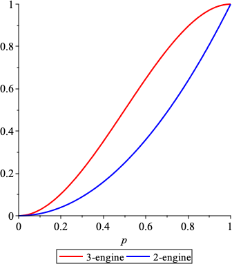
Figure 5.1: Failure probability for the 2-engine and 3-engine planes.
(Taken from [8]) Air traffic control is a safety-related activity – each piece of equipment is designed to the highest safety standards and in many cases duplicate equipment is provided so that if one item fails another takes over.
A new system is to be provided passing information from Heathrow Airport to Terminal Control at West Drayton. As part of the system design a decision has to be made as to whether it is necessary to provide duplication. The new system takes data from the Ground Movements Radar (GMR) at Heathrow, combines this with data from the National Airspace System NAS, and sends the output to a display at Terminal Control (a conceptual model is shown in Figure 5.2).
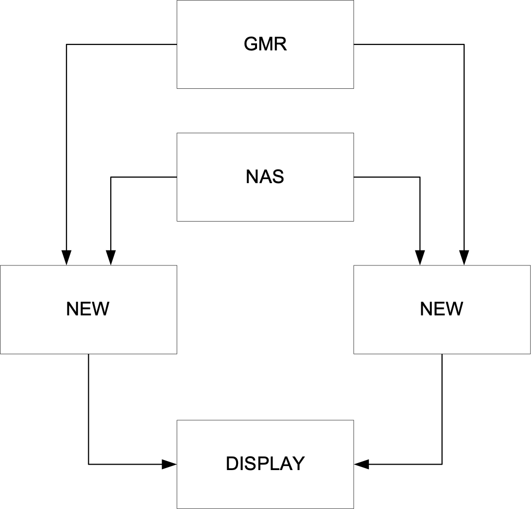
Figure 5.2: Conceptual model of air traffic control security system.
For all existing systems, records of failure are kept and an experimental probability of failure is calculated annually using the previous 4 years.
The reliability of a system is defined as \(R=1 - P\), where \(P=P(\text{failure})\).
\(R_{\text{GMR}} = R_{\text{NAS}} = 0.9999\) (i.e., \(1\) failure in \(10,000\) hours).
the components’ failure probabilities are independent.
For the system above, if a single module is introduced the reliability of the system (STD – single thread design) is \[R_{\text{STD}}=R_{\text{GMR}} \times R_{\text{NEW}} \times R_{\text{NAS}}.\]
If the module is duplicated, the reliability of this dual thread design is \[R_{\text{DTD}}=R_{\text{GMR}} \times (1 - (1 - R_{\text{NEW}} )^2) \times R_{\text{NAS}}.\] Duplicating the module causes an improvement in reliability of \[\rho=\frac{R_{\text{DTD}}}{R_{\text{STD}}}=\frac{(1 - (1 - R_{\text{NEW}} )^2)}{R_{\text{NEW}}} \times 100\%\,.\]
For the module, no historical data is available. Instead, we work out the improvement achieved by using the dual thread design for various values of \(R_{\text{NEW}}\).
\(R_{\text{NEW}}\) 0.1 0.2 0.5 0.75 0.99 0.999 0.9999 0.99999 \(\rho\) (%) 190 180 150 125 101 100.1 100.01 100.001 If the module is very unreliable (i.e., \(R_{\text{NEW}}\) is small), then there is a significant benefit in using the dual thread design (\(\rho\) is large).7
If the new module is as reliable as and , that is, if \[R_{\text{GMR}} =R_{\text{NEW}} = R_{\text{NAS}} = 0.9999,\] then the single thread design has a combined reliability of \(0.9997\) (i.e., \(3\) failures in \(10,000\) hours), whereas the dual thread design has a combined reliability of \(0.9998\) (i.e., \(2\) failures in \(10,000\) hours).
If the probability of failure is independent for each component, we could conclude from this that the reliability gain from a dual thread design probably does not justify the extra cost.
In the last two examples, we had to make additional assumptions in order to answer the questions – this is often the case in practice.
Conditional Probability
It is easier to understand independence of events through the conditional probability of an event \(B\) given that another event \(A\) has occurred, defined by as \[\begin{aligned} {P(B \mid A)}=\frac{P(A\cap B)}{P(A)}\,.\end{aligned}\] Note that this definition only makes sense when “\(A\) can happen” i.e., \(P(A)>0\). If \(P(A)P(B)>0\), then \[P(A\cap B)=P(A)\times P(B \mid A)=P(B)\times P(A \mid B)=P(B\cap A);\] \(A\) and \(B\) are thus independent if \(P(B \mid A)=P(B)\) and \(P(A \mid B)=P(A)\).
Examples:
From a group of 100 people, 1 is selected. What is the probability that this person has high blood pressure (HBP)?
Answer: if we know nothing else about the population, this is an (unconditional) probability, namely \[P(\text{HBP})=\frac{\# \text{individuals with HBP in the population}}{100}\,.\]
If instead we first filter out all people with low cholesterol level, and then select 1 person. What is the probability that this person has HBP?
Answer: this is the conditional probability \[P(\text{HBP} \mid \text{high cholesterol});\] the probability of selecting a person with HBP, given high cholesterol levels, presumably different from \(P(\text{HBP} \mid \text{low cholesterol})\).
A sample of \(249\) individuals is taken and each person is classified by blood type and tuberculosis (TB) status.
O A B AB Total TB \(34\) \(37\) \(31\) \(11\) \(113\) no TB \(55\) \(50\) \(24\) \(7\) \(136\) Total \(89\) \(87\) \(55\) \(18\) \(249\) The (unconditional) probability that a random individual has TB is \(P(\text{TB})=\frac{\# \text{TB}}{249}=\frac{113}{249} = 0.454\). Among those individuals with type B blood, the (conditional) probability of having TB is \[P(\text{TB} \mid \text{type {\bf B}})= \frac{P(\text{TB}\cap \text{type {\bf B}})}{P(\text{type {\bf B}})}=\frac{31}{55} = \frac{31/249}{55/249}= 0.564.\]
A family has two children (not twins). What is the probability that the youngest child is a girl given that at least one of the children is a girl? Assume that boys and girls are equally likely to be born.
Answer: let \(A\) and \(B\) be the events that the youngest child is a girl and that at least one child is a girl, respectively: \[A=\{\text{GG},\text{BG}\} \quad\mbox{and}\quad B=\{\text{GG},\text{BG},\text{GB}\},\] \(A\cap B=A.\) Then \(P(A \mid B)=\frac{P(A\cap B)}{P(B)} = \frac{P(A)}{P(B)}=\frac{2/4}{3/4}=\frac{2}{3}\) (and not \(\frac12\), as might naively be believed).
Incidentally, \(P(A\cap B)=P(A)\neq P(A)\times P(B)\), which means that \(A\) and \(B\) are not independent events.
Law of Total Probability
Let \(A\) and \(B\) be two events. From set theory, we have \[B=(A\cap B)\cup (\overline{A}\cap B),\] as illustrated in Figure 5.3.
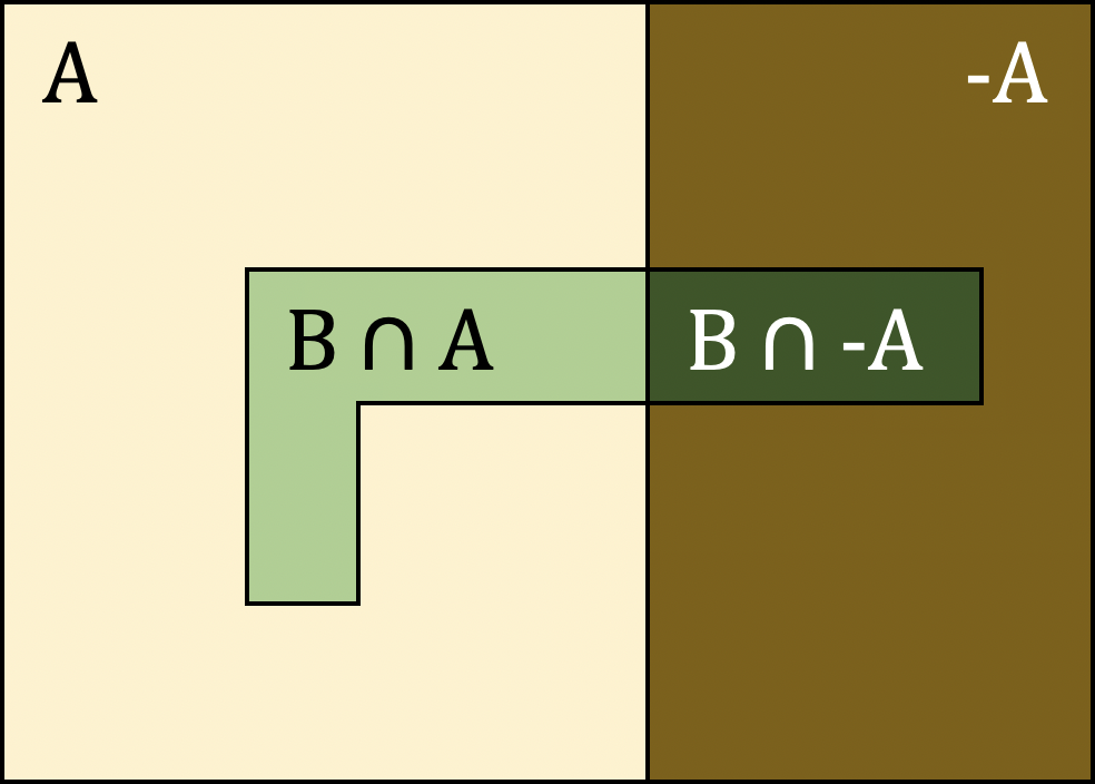
Figure 5.3: Decomposition of \(B\) via \(A\).
Note that \(A\cap B\) and \(\overline{A}\cap B\) are mutually exclusive, so that, according to Axiom \(\textbf{A4}\), we have \[P(B)=P(A\cap B)+P(\overline{A}\cap B).\] Now, assuming that \(\text{Var}nothing \neq A \neq \mathcal{S}\), \[P(A\cap B) = P(B \mid A)P(A) \quad\mbox{and} \quad P(\overline{A}\cap B)=P(B \mid \overline{A})P(\overline{A}),\] so that \[P(B) = P(B \mid A)P(A)+P(B \mid \overline{A})P(\overline{A}).\] This generalizes as follows: if \(A_1,...A_k\) are mutually exclusive and exhaustive (i.e., \(A_i\cap A_j=\text{Var}nothing\) for all \(i\neq j\) and \(A_1\cup ....\cup A_k=\mathcal{S})\), then for any event \(B\) \[\begin{aligned} P(B)&=\sum_{j=1}^kP(B \mid A_j)P(A_j)\\&=P(B \mid A_1)P(A_1 )+...+P(B \mid A_k)P(A_k).\end{aligned}\]
Example: use the Law of Total Probability (rule above) to compute \(P(\text{TB})\) using the data from the previous example.
Answer: the blood types \(\{\textbf{O},\textbf{A},\textbf{B},\textbf{AB}\}\) form a mutually exclusive partition of the population, with \[P(\textbf{O})=\frac{89}{249},\ P(\textbf{A})=\frac{87}{249},\ P(\textbf{B})=\frac{55}{249},\ P(\textbf{AB})=\frac{18}{249}.\] It is easy to see that \(P(\textbf{O})+ P(\textbf{A})+P(\textbf{B})+ P(\textbf{AB})=1\). Furthermore, \[\begin{aligned} P(\text{TB} \mid \textbf{O})&=\textstyle{\frac{P(\text{TB}\cap\textbf{O})}{P(\textbf{O})}=\frac{34}{89},\ P(\text{TB} \mid \textbf{A})=\frac{P(\text{TB}\cap\textbf{A})}{P(\textbf{A})}=\frac{37}{87}},\\ P(\text{TB} \mid \textbf{B})&=\textstyle{\frac{P(\text{TB}\cap\textbf{B})}{P(\textbf{B})}=\frac{31}{55},\ P(\text{TB} \mid \textbf{AB})=\frac{P(\text{TB}\cap\textbf{AB})}{P(\textbf{AB})}=\frac{11}{18}}.\end{aligned}\]
According to the law of total probability, \[\begin{aligned} P(\text{TB})=P(\text{TB} &\mid \textbf{O})P(\textbf{O})+P(\text{TB} \mid \textbf{A})P(\textbf{A})\\ & +P(\text{TB} \mid \textbf{B})P(\textbf{B})+P(\text{TB} \mid \textbf{AB})P(\textbf{AB}), \end{aligned}\] so that \[\begin{aligned} P(\text{TB})&=\frac{34}{89}\cdot\frac{89}{249}+\frac{37}{87}\cdot\frac{87}{249}+\frac{31}{55}\cdot\frac{55}{249}+\frac{11}{18}\cdot\frac{18}{249}\\ &=\frac{34+37+31+11}{249}=\frac{113}{249}=0.454, \end{aligned}\] which matches with the result of the previous example.
5.1.7 Bayes’ Theorem
After an experiment generates an outcome, we are often interested in the probability that a certain condition was present given an outcome (or that a particular hypothesis was valid, say).
We have noted before that if \(P(A)P(B)>0\), then \[P(A\cap B)=P(A)\times P(B \mid A)=P(B)\times P(A \mid B)=P(B\cap A);\] this can be re-written as Bayes’ Theorem: \[P(A \mid B)=\frac{P(B \mid A) \times P(A)}{P(B)}.\] Bayes’ Theorem is a powerful tool in probability analysis, but it is a simple corollary of the rules of probability.
Central Data Analysis Question
Given everything that was known prior to the experiment, does the collected/observed data support (or invalidate) the hypothesis/presence of a certain condition?
The problem is that this is usually impossible to compute directly. Bayes’ Theorem offers a possible solution: \[\begin{aligned} P(\text{hypothesis} \mid \text{data})&=\frac{P(\text{data} \mid \text{hypothesis})\times P(\text{hypothesis})}{P(\text{data})} \\ &\propto P(\text{data} \mid \text{hypothesis})\times P(\text{hypothesis}),\end{aligned}\] in which the terms on the right might be easier to compute than the term on the left.
Bayesian Vernacular
In Bayes’ Theorem:
\(P(\text{hypothesis})\) is the probability of the hypothesis being true prior to the experiment (called the prior);
\(P(\text{hypothesis} \mid \text{data})\) is the probability of the hypothesis being true once the experimental data is taken into account (called the posterior);
\(P(\text{data} \mid \text{hypothesis})\) is the probability of the experimental data being observed assuming that the hypothesis is true (called the likelihood).
The theorem is often presented as \(\text{posterior} \propto \text{likelihood} \times \text{prior}\), which is to say, beliefs should be updated in the presence of new information.
Formulations
If \(A,B\) are events for which \(P(A)P(B)>0\), then Bayes’ Theorem can be re-written, using the law of total probability, as \[P(A \mid B)=\frac{P(B \mid A)P(A)}{P(B)}=\frac{P(B \mid A)P(A)}{P(B \mid A)P(A)+P(B \mid \overline{A})P(\overline{A})},\] or, in the general case where \(A_1,...A_k\) are mutually exclusive and exhaustive events, then for any event \(B\) and for each \(1\leq i\leq k\), \[\begin{aligned} P(A_i \mid B)&= \frac{P(B \mid A_i)P(A_i)}{P(B)}\\ &=\frac{P(B \mid A_i)P(A_i)}{P(B \mid A_1)P(A_1 )+...+P(B \mid A_k)P(A_k)}.\end{aligned}\]
Examples:
In 1999, Nissan sold three car models in North America: Sentra (S), Maxima (M), and Pathfinder (PA). Of the vehicles sold that year, \(50\%\) were S, \(30\%\) were M and \(20\%\) were PA. In the same year \(12\%\) of the S, \(15\%\) of the M, and \(25\%\) of the PA had a particular defect \(D\).
If you own a 1999 Nissan, what is the probability that it has the defect?
in the language of conditional probability, \[\begin{aligned} P(\text{S})&=0.5, \ P(\text{M})=0.3, \ P(\text{Pa})=0.2, \\ P(D \mid \text{S})&=0.12, \ P(D \mid \text{M})=0.15, \ P(D \mid \text{PA})=0.25, \end{aligned}\]so that \[\begin{aligned} P(&D)=P(D \mid \text{S})\times P(\text{S})+P(D \mid \text{M})\times P(\text{M})\\&+P(D \mid \text{Pa})\times P(\text{Pa}) \\ &=0.12\cdot 0.5+0.15\cdot 0.3+0.25\cdot 0.2\\&= 0.155 = 15.5\%.\end{aligned}\]
If a 1999 Nissan has defect \(D\), what model is it likely to be?
in the first part we computed the total probability \(P(D)\); in this part, we compare the posterior probabilities \(P(\text{M} \mid D)\), \(P(\text{S} \mid D)\), and \(P(\text{Pa} \mid D)\) (and not the priors!), computed using Bayes’ Theorem: \[\begin{aligned} P(\text{S} \mid D)&=\textstyle{\frac{P(D \mid \text{S})P(\text{S})}{P(D)}=\frac{0.12\times 0.5}{0.155}\approx 38.7\%} \\ P(\text{M} \mid D)&=\textstyle{\frac{P(D \mid \text{M})P(\text{M})}{P(D)}=\frac{0.15\times 0.3}{0.155}\approx 29.0\%} \\ P(\text{Pa} \mid D)&=\textstyle{\frac{P(D \mid \text{Pa})P(\text{Pa})}{P(D)}=\frac{0.25\times 0.2}{0.155}\approx 32.3\%} \end{aligned}\] Even though Sentras are the least likely to have the defect \(D\), their overall prevalence in the population carry them over the hump.
Suppose that a test for a particular disease has a very high success rate. If a patient
has the disease, the test reports a ‘positive’ with probability 0.99;
does not have the disease, the test reports a ‘negative’ with prob 0.95.
Assume that only 0.1% of the population has the disease. What is the probability that a patient who tests positive does not have the disease?
Answer: Let \(D\) be the event that the patient has the disease, and \(A\) be the event that the test is positive. The probability of a true positive is \[\begin{aligned} P(D \mid A)&=\frac{P(A \mid D)P(D)}{P(A \mid D)P(D)+P(A \mid D^c)P(D^c)}\\ &=\frac{0.99\times 0.001}{0.99\times 0.001 + 0.05\times 0.999}\approx 0.019.\end{aligned}\] The probability of a false positive is thus \(1-0.019\approx 0.981\). Despite the apparent high accuracy of the test, the incidence of the disease is so low (\(1\) in a \(1000\)) that the vast majority of patients who test positive (\(98\) in \(100\)) do not have the disease.
The \(2\) in \(100\) who are true positives still represent \(20\) times the proportion of positives found in the population (before the outcome of the test is known).[It is important to remember that when dealing with probabilities, both the likelihood and the prevalence have to be taken into account.]
(Monty Hall Problem) On a game show, you are given the choice of three doors. Behind one of the doors is a prize; behind the others, dirty and smelly rubbish bins (as is skillfully rendered in Figure 5.4).
You pick a door, say No. 1, and the host, who knows what is behind the doors, opens another door, say No. 3, behind which is a bin. She then says to you, “Do you want to switch from door No. 1 to No. 2?”
Is it to your advantage to do so?

Figure 5.4: The Monty Hall set-up (personal file, but that was probably obvious).
Answer: in what follows, let and be the events that switching to another door is a successful strategy and that the prize is behind the original door, respectively.
Let’s first assume that the host opens no door. What is the probability that switching to another door in this scenario would prove to be a successful strategy?
If the prize is behind the original door, switching would succeed 0% of the time: \[P(\text{S} \mid \text{D})=0.\] Note that the prior is \(P(\text{D})=1/3\).
If the prize is not behind the original door, switching would succeed 50% of the time: \[P(\text{S} \mid \text{D}^c)=1/2.\] Note that the prior is \(P(\text{D}^c)=2/3\). Thus, \[\begin{aligned} P(&\text{S}) = P(\text{S} \mid \text{D}) P(\text{D}) +P(\text{S} \mid \text{D}^c)P(\text{D}^c) \\ & =0\cdot \frac{1}{3}+\frac{1}{2}\cdot \frac{2}{3} \approx 33\%. \quad\end{aligned}\]
Now let’s assume that the host opens one of the other two doors to show a rubbish bin. What is the probability that switching to another door in this scenario would prove to be a successful strategy?
If the prize is behind the original door, switching would succeed 0% of the time: \[P(\text{S} \mid \text{D})=0.\] Note that the prior is \(P(\text{D})=1/3\).
If the prize is not behind the original door, switching would succeed 100% of the time: \[P(\text{S} \mid \text{D}^c)=1.\] Note that the prior is \(P(\text{D}^c)=2/3\). Thus, \[\begin{aligned} P(&\text{S}) = P(\text{S} \mid \text{D}) P(\text{D}) +P(\text{S} \mid \text{D}^c)P(\text{D}^c) \\&=0\cdot \frac{1}{3}+1\cdot \frac{2}{3} \approx 67\%. \quad\end{aligned}\]
If no door is opened, switching is not a winning strategy, resulting in success only 33% of the time. If a door is opened, however, switching becomes the winning strategy, resulting in success 67% of the time.
This problem has attracted a lot of attention over the years due to its counter-intuitive result, but there is no paradox when we understand conditional probabilities.
The following simulations may make it easier to see.
Perhaps you would rather see what happens in practice: if you could pit two players against one another (one who never switches and one who always does so) in a series of Monty Hall games, which one would come out on top in the longrun?
# number of games (if N is too small, we don't have long-run behaviour)
N=500

# fixing the seed for replicability purposes
set.seed(1234)

# placing the prize behind one of the 3 doors for each game
locations = sample(c("A","B","C"), N, replace = TRUE)

# verification that the prize gets placed behind each door roughly 33% of the time
table(locations)/N
locations
A B C
0.302 0.344 0.354 # getting the playerto select a door for each of the N games (in practice, should be independent of where the prize actually is)
player.guesses = sample(c("A","B","C"), N, replace = TRUE)
# create a data frame telling the analyst where the prize is, and what door the player has selected
games = data.frame(locations, player.guesses)
head(games)
# how often does the player guess correctly, before a door is opened (should be about 33%)
table(games$locations==games$player.guesses) locations player.guesses
1 B B
2 B B
3 A B
4 C C
5 A C
6 A A
FALSE TRUE
333 167 # initialize the process to find out which door the host will open
games$open.door <- NA
# for each game, the host opens a door which is not the one selected by the player, nor the one behind which the prize is found
# the union() call enumerates the doors that the host cannot open
# the setdiff() call finds the complementof the doors that thehost cannotopen (i.e.: the doors that she can open)
# the sample() call picks one of those doors
for(j in 1:N){
games$open.door[j] <- sample(setdiff(c("A","B","C"), union(games$locations[j],games$player.guesses[j])), 1)
}
head(games) locations player.guesses open.door
1 B B C
2 B B C
3 A B C
4 C C A
5 A C B
6 A A B# if the player neverswitches, they win whenever they had originally guessed the location of the prize correctly
games$no.switch.win <- games$player.guess==games$locations
# let's find which doorthe playerwould have selected if they alwaysswitched (the doorthatis neither the location of the prize nor theonethey hadoriginally selected)
games$switch.door <- NA
for(j in 1:N){
games$switch.door[j] <- sample(setdiff(c("A","B","C"), union(games$open.door[j],games$player.guesses[j])), 1)
}
# if the player always switches, they win whenever their switched guess is wheretheprize is located
games$switch.win <- games$switch.door==games$locations
head(games) locations player.guesses open.door no.switch.win switch.door switch.win
1 B B C TRUE A FALSE
2 B B C TRUE A FALSE
3 A B C FALSE A TRUE
4 C C A TRUE B FALSE
5 A C B FALSE A TRUE
6 A A B TRUE C FALSE# chance of winning by not switching
table(games$no.switch.win)/N
# chance of winning by switching
table(games$switch.win)/N
FALSE  TRUE
0.666 0.334

FALSE  TRUE
0.334 0.666
Pretty wild, eh?
5.2 Discrete Distributions
The principles of probability theory introduced in the previous section are simple, and they are always valid. In this section and the next, we will see how some of the associated computations can be made easier with the use of distributions.
5.2.1 Random Variables and Distributions
Recall that, for any random “experiment”, the set of all possible outcomes is denoted by \({\cal S}\). A random variable (r.v.) is a function \(X:\mathcal{S}\to \mathbb{R}\), which is to say, it is a rule that associates a (real) number to every outcome of the experiment; \({\cal S}\) is the domain of the r.v. \(X\) and \(X(\mathcal{S})\subseteq \mathbb{R}\) is its range.
A probability distribution function (p.d.f.) is a function \(f:\mathbb{R}\to \mathbb{R}\) which specifies the probabilities of the values in the range \(X(\mathcal{S})\).
When \(\mathcal{S}\) is discrete,8 we say that \(X\) is a discrete r.v. and the p.d.f. is called a probability mass function (p.m.f.).
Notation
Throughout, we use the following notation:
capital roman letters (\(X\), \(Y\), etc.) denote r.v., and
corresponding lower case roman letters (\(x\), \(y\), etc.) denote generic values taken by the r.v.
A discrete r.v.can be used to define events – if \(X\) takes values \(X(\mathcal{S})=\{x_i\}\), then we can define the events \[A_i=\left\{s\in \mathcal{S}: X(s)=x_i \right\}:\]
the p.m.f. of \(X\) is \[f(x)=P\left( \left\{s\in \mathcal{S}: X(s)=x \right\} \right):=P(X=x);\]
its cumulative distribution function (c.d.f.) is \[F(x)=P(X\leq x).\]
Properties
If \(X\) is a discrete random variable with p.m.f. \(f(x)\) and c.d.f. \(F(x)\), then
\(0<f(x)\leq 1\) for all \(x\in X(\mathcal{S})\);
\(\sum_{s\in \mathcal{S}}f(X(s))=\sum_{x\in X(\mathcal{S})}f(x)=1\);
for any event \(A\subseteq \mathcal{S}\), \(P(X\in A)=\sum_{x\in A}f(x)\);
for any \(a,b\in \mathbb{R}\), \[\begin{aligned} P(a<X)&=1-P(X\leq a)=1-F(a) \\ P(X<b)&=P(X\leq b)-P(X=b)=F(b)-f(b)\end{aligned}\]
for any \(a,b\in \mathbb{R}\), \[\begin{aligned} P(a\leq X)&=1-P(X<a)\\&=1-(P(X\leq a)-P(X=a)) \\ &=1-F(a)+f(a) \end{aligned}\]
We can use these results to compute the probability of a discrete r.v. \(X\) falling in various intervals: \[\begin{aligned} P(a<X\leq b)&=P(X\leq b)-P(X\leq a)\\&=F(b)-F(a) \\ P(a\leq X\leq b)&=P(a<X\leq b)+P(X=a)\\&=F(b)-F(a)+f(a) \\ P(a<X< b)&=P(a<X\leq b)-P(X=b)\\&=F(b)-F(a)-f(b) \\ P(a\leq X<b)&=P(a\leq X\leq b)-P(X=b)\\&=F(b)-F(a)+f(a)-f(b) \end{aligned}\]
Examples:
Flip a fair coin – the outcome space is \(\mathcal{S}=\{\text{Head}, \text{Tail}\}\). Let \(X:S\to\mathbb{R}\) be defined by \(X(\text{Head})=1\) and \(X(\text{Tail})=0\). Then \(X\) is a discrete random variable (as a convenience, we write \(X=1\) and \(X=0\)).
If the coin is fair, the p.m.f. of \(X\) is \(f:\mathbb{R}\to \mathbb{R}\), where \[\begin{aligned} f(0)&=P(X=0)=1/2,\ f(1)=P(X=1)=1/2,\\ f(x)&=0 \text{ for all other $x$}.\end{aligned}\]
Roll a fair die – the outcome space is \(\mathcal{S}=\{1,\ldots, 6\}\). Let \(X:\mathcal{S}\to\mathbb{R}\) be defined by \(X(i)=i\) for \(i=1,\ldots, 6\). Then \(X\) is a discrete r.v.
If the die is fair, the p.m.f. of \(X\) is \(f:\mathbb{R}\to \mathbb{R}\), where \[\begin{aligned} f(i)&=P(X=i)=1/6, \ \text{for }i=1,\ldots, 6, \\ f(x)&=0 \text{ for all other $x$}.\end{aligned}\]
For the random variable \(X\) from the previous example, the c.d.f. is \(F:\mathbb{R}\to\mathbb{R}\), where \[\begin{aligned} F(x)&=P(X\leq x)= \begin{cases} 0 & \text{if $x<1$} \\ i/6 & \text{if $i\leq x<i+1$, $i=1,\ldots, 6$} \\ 1 & \text{if $x\geq 6$} \end{cases}\end{aligned}\]
For the same random variable, we can compute the probability \(P(3\le X\le 5)\) directly: \[\begin{aligned} P(3\leq X\leq 5)&=P(X=3)+P(X=4)+P(X=5)\\&=\textstyle{\frac{1}{6}+\frac{1}{6}+\frac{1}{6}=\frac{1}{2}},\end{aligned}\] or we can use the c.d.f.: \[\textstyle{P(3\leq X\leq 5)=F(5)-F(3)+f(3)=\frac{5}{6}-\frac{3}{6}+\frac{1}{6}=\frac{1}{2}.}\]
The number of calls received over a specific time period, \(X\), is a discrete random variable, with potential values \(0,1,2,\ldots\).
Consider a \(5-\)card poker hand consisting of cards selected at random from a \(52-\)card deck. Find the probability distribution of \(X\), where \(X\) indicates the number of red cards (\(\diamondsuit\) and \(\heartsuit\)) in the hand.
Answer: in all there are \(\binom{52}{5}\) ways to select a \(5-\)card poker hand from a \(52-\)card deck. By construction, \(X\) can take on values \(x=0,1,2,3,4,5\).
If \(X=0\), then none of the \(5\) cards in the hands are \(\diamondsuit\) or \(\heartsuit\), and all of the \(5\) cards in the hands are \(\spadesuit\) or \(\clubsuit\). There are thus \(\binom{26}{0}\cdot \binom{26}{5}\) \(5-\)card hands that only contain black cards, and \[P(X=0)=\frac{\binom{26}{0} \cdot \binom {26}{5}}{\binom {52}{5}}.\] In general, if \(X=x\), \(x=0,1,2,3,4,5\), there are \(\binom{26}{x}\) ways of having \(x\) \(\diamondsuit\) or \(\heartsuit\) in the hand, and \(\binom{26}{5-x}\) ways of having \(5-x\) \(\spadesuit\) and \(\clubsuit\) in the hand, so that \[\begin{aligned} f(x)&=P(X=x)=\begin{cases}\frac{\binom{26}{x}\cdot \binom {26}{5-x}}{\binom{52}{5}},\ x=0,1,2,3,4,5; \\ 0 \text{ otherwise}\end{cases} \end{aligned}\]
Find the c.d.f.of a discrete random variable \(X\) with p.m.f. \(f(x)=0.1x\) if \(x=1,2,3,4\) and \(f(x)=0\) otherwise.
Answer: \(f(x)\) is indeed a p.m.f. as \(0<f(x)\leq 1\) for all \(x\) and \[\sum_{x=1}^40.1x=0.1(1+2+3+4)=0.1\frac{4(5)}{2}=1.\] Computing \(F(x)=P(X\leq x)\) yields \[F(x)=\begin{cases} 0 & \text{if $x<1$} \\ 0.1 & \text{if $1\leq x<2$} \\ 0.3 & \text{if $2\leq x<3$} \\ 0.6 & \text{if $3\leq x<4$} \\ 1 & \text{if $x\geq 4$} \end{cases}\]
The p.m.f. and the c.m.f. for this r.v. are shown in Figure 5.5.
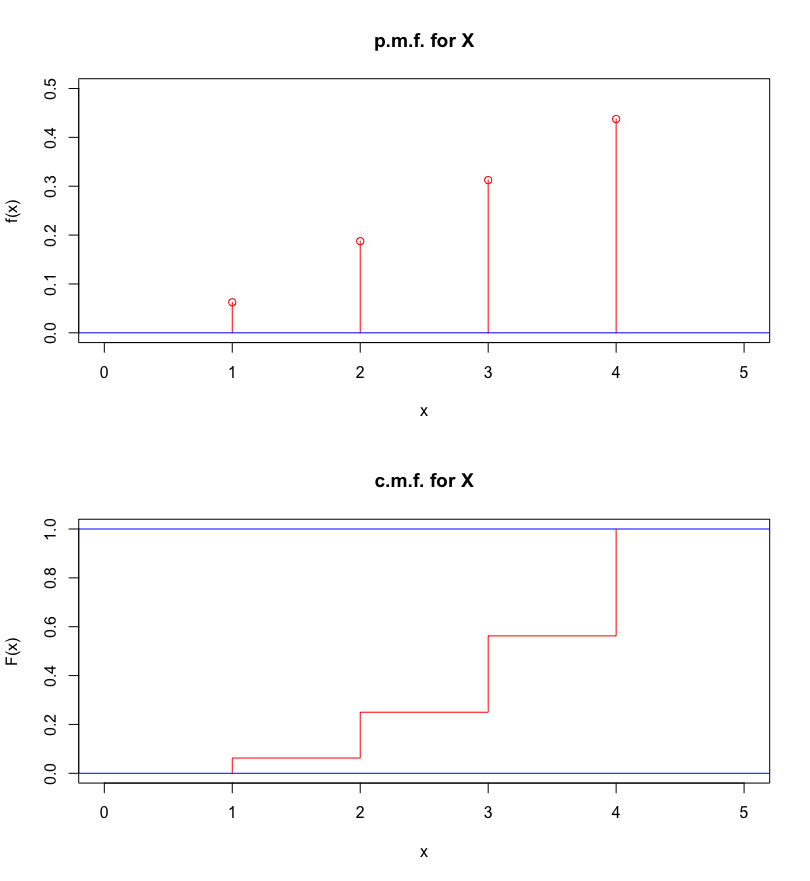
Figure 5.5: P.m.f. and c.m.f. for the r.v. \(X\) defined above.
5.2.2 Expectation of a Discrete Random Variable
The expectation of a discrete random variable \(X\) is \[{\text{E} [X]}=\sum_x x\cdot P(X=x)=\sum_{x}xf(x)\,,\] where the sum extends over all values of \(x\) taken by \(X\).
The definition can be extended to a general function of \(X\): \[\text{E}[u(X)]=\sum_{x}u(x)P(X=x)=\sum_xu(x)f(x).\] As an important example, note that \[\text{E}[X^2]=\sum_x x^2P(X=x)=\sum_xx^2f(x).\]
Examples:
What is the expectation on the roll \(Z\) of \(6-\)sided die?
Answer: if the die is fair, then \[\begin{aligned} \text{E} [Z]&=\sum_{z=1}^6z\cdot P(Z=z) =\frac{1}{6}\sum_{z=1}^6z\\&=\frac{1}{6}\cdot\frac{6(7)}{2}=3.5.\end{aligned}\]
For each \(1\$\) bet in a gambling game, a player can win \(3\$\) with probability \(\frac{1}{3}\) and lose \(1\$\) with probability \(\frac{2}{3}\). Let \(X\) be the net gain/loss from the game. Find the expected value of the game.
Answer: \(X\) can take on the value \(2\$\) for a win and \(-2\$\) for a loss (outcome \(-\) bet). The expected value of \(X\) is thus \[\text{E}[X]=2\cdot\frac{1}{3}+(-2)\cdot\frac{2}{3}=-\frac{2}{3}.\]
If \(Z\) is the number showing on a roll of a fair \(6-\)sided die, find \(\text{E} [Z^2]\) and \(\text{E} [(Z-3.5)^2]\).
Answer: \[\begin{aligned} \text{E}[Z^2]&= \sum_z z^2P(Z=z) = \frac{1}{6}\sum_{z=1}^6z^2\\ &=\frac16(1^2+\cdots+6^2)=\frac{91}{6}\\ \text{E}[(Z&-3.5)^2]=\sum_{z=1}^6(z-3.5)^2P(Z=z)\\&=\frac{1}{6}\sum_{z=1}^6(z-3.5)^2 \\ &=\frac{(1-3.5)^2+\cdots+(6-3.5)^2}{6}=\frac{35}{12}.\end{aligned}\]
The expectation of a random variable is simply the average value that it takes, over all possible values.
Mean and Variance
We can interpret the expectation as the average or the mean of \(X\), which we often denote by \(\mu=\mu_X\). For instance, in the example of the fair die, \[\mu_Z=\text{E}[Z]=3.5\]
Note that in the final example, we could have written \[\text{E}[ (Z-3.5)^2 ]=\text{E}[ (Z-\text{E}[Z])^2 ].\] This is an important quantity associated to a random variable \(X\), its variance \(\text{Var}[X]\).
The variance of a discrete random variable \(X\) is the expected squared difference from the mean: \[\begin{aligned} \text{Var} (X)&= \text{E} [ (X-\mu_X)^2]= \sum_{x} (x-\mu_X)^2P(X=x)\\&=\sum_{x}\left(x^2-2x\mu_X+\mu_X^2\right)f(x) \\&= \sum_{x}x^2f(x)-2\mu_X\sum_{x}xf(x)+\mu_X^2\sum_{x}f(x)\\&= \text{E}[X^2]-2\mu_X\mu_X+\mu_X^2\cdot 1 \\ &=\text{E}[X^2]-\mu_X^2.\end{aligned}\] This is also sometimes written as \(\text{Var}[X]=\text{E}[X^2]-\text{E}^2[X]\).
Standard Deviation
The standard deviation of a discrete random variable \(X\) is defined directly from the variance: \[\text{SD}[X]=\sqrt{\text{Var} [X]}\,.\] The mean is a measure of centrality and it gives an idea as to where the bulk of a distribution is located; the variance and standard deviation provide information about the spread – distributions with higher variance/SD are more spread out about the average.
Example: let \(X\) and \(Y\) be random variables with the following p.d.f.
| \(x\) | \(P(X=x)\) | \(y\) | \(P(Y=y)\) |
|---|---|---|---|
| \(-2\) | \(1/5\) | \(-4\) | \(1/5\) |
| \(-1\) | \(1/5\) | \(-2\) | \(1/5\) |
| \(0\) | \(1/5\) | \(0\) | \(1/5\) |
| \(1\) | \(1/5\) | \(2\) | \(1/5\) |
| \(2\) | \(1/5\) | \(4\) | \(1/5\) |
Compute the expected values and compare the variances.
Answer: we have \(\text{E} [X]=\text{E} [Y]=0\) and \[2=\text{Var}[X]<\text{Var}[Y]=8,\] meaning that we would expect both distributions to be centered at \(0\), but \(Y\) should be more spread-out than \(X\) (because its variance is greater, see Figure 5.6).
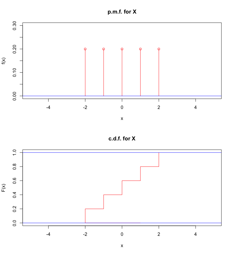
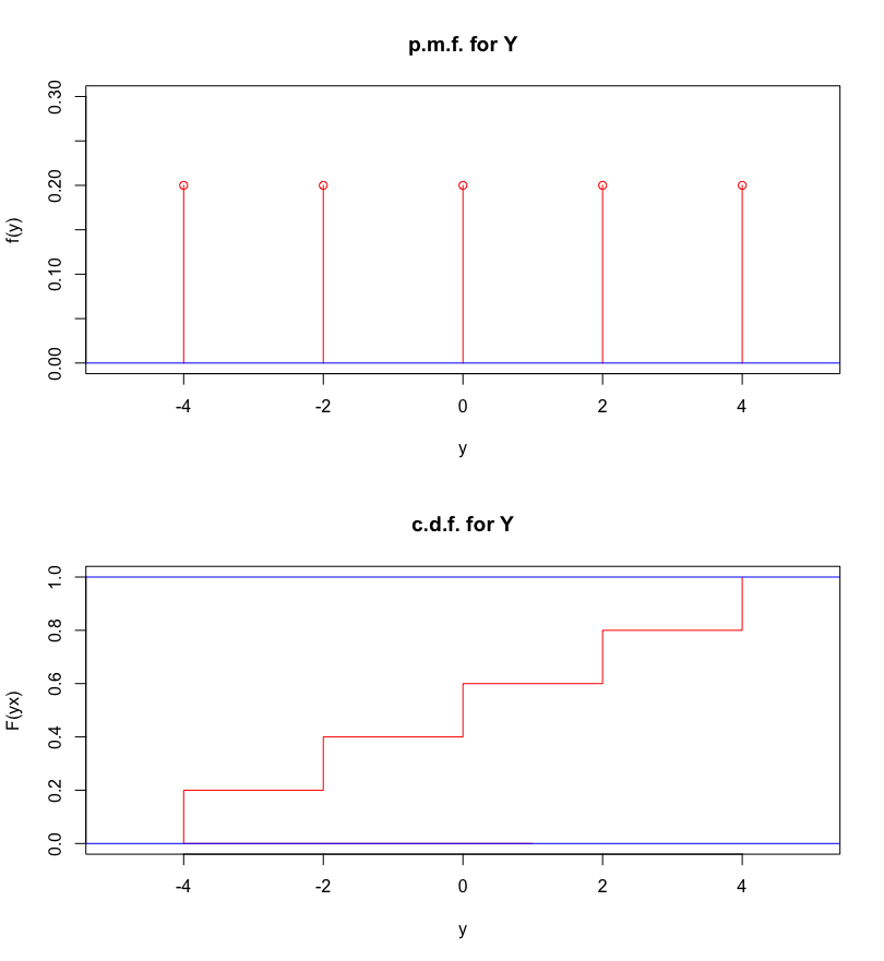
Figure 5.6: R.v. \(X\) (left) and \(Y\) (right), defined above.
Properties
Let \(X,Y\) be random variables and \(a\in \mathbb{R}\). Then
\(\text{E} [aX]=a\text{E}[X]\);
\(\text{E} [X+a]= \text{E}[X]+a\);
\(\text{E} [X+Y]=\text{E}[X]+\text{E}[Y]\);
in general, \(\text{E} [XY]\neq \text{E}[X]\text{E}[Y]\);
\(\text{Var}[aX]=a^2\text{Var}[X]\), \(\text{SD}[aX]=|a|\text{SD}[X]\);
\(\text{Var}[X+a]=\text{Var} [X]\), \(\text{SD}[X+a]=\text{SD} [X]\).
5.2.3 Binomial Distributions
Recall that the number of unordered samples of size \(r\) from a set of size \(n\) is \[_nC_r=\binom{n}{r}=\frac{n!}{(n-r)!r!}.\]
Examples
\(2!\times 4!=(1\times 2)\times (1\times 2\times 3\times 4)=48\), but \((2\times 4)!=8!=40320\).
\(\binom 5 1=\frac{5!}{1!\times 4!}=\frac{1\times 2\times 3\times 4\times 5}{1\times (1\times 2\times 3\times 4)}=\frac{5}{1}=5\).
In general: \(\binom n 1=n\) and\(\binom n 0=1\).
\(\binom 6 2=\frac{6!}{2!\times 4!}=\frac{4!\times 5\times 6}{2!\times 4!}=\frac{5\times 6}{2}=15\).
\(\binom {27} {22}=\frac{27!}{22!\times 5!}=\frac{22!\times 23\times 24\times 25\times 26\times 27}{5!\times 22!}=\frac{23\times 24\times 25\times 26\times 27}{120}\).
Binomial Experiments
A Bernoulli trial is a random experiment with two possible outcomes, “success" and”failure". Let \(p\) denote the probability of a success.
A binomial experiment consists of \(n\) repeated independent Bernoulli trials, each with the same probability of success, \(p\), such as:
female/male births (perahps not truly independent, but often treated as such);
satisfactory/defective items on a production line;
sampling with replacement with two types of item,
etc.
Probability Mass Function
In a binomial experiment of \(n\) independent events, each with probability of success \(p\), the number of successes \(X\) is a discrete random variable that follows a binomial distribution with parameters \((n,p)\): \[f(x)=P(X=x)=\binom nx p^x(1-p)^{n-x}\,,\ \text{ for $x=0,1,2,\ldots,n$.}\] This is often abbreviated to “\(X\sim\mathcal{B}(n,p)\)”.
If \(X\sim \mathcal{B}(1,p)\), then \(P(X=0)=1-p\) and \(P(X=1)=p\), so \[\text{E} [X]=(1-p)\cdot0 + p\cdot1=p\,.\]
Expectation and Variance
If \(X\sim \mathcal{B}(n,p)\), it can be shown that \[\text{E} [X]= \sum_{x=0}^n xP(X=x) =np,\] and \[\text{Var}[X]= \text{E}\left[(X-np)^2 \right] = \sum_{x=0}^n (x-np)^2 P(X=x)=np(1-p)\] (we will eventually see an easier way to derive these formulas by interpreting \(X\) as a sum of other discrete random variables).
Recognizing that certain situations can be modeled via a distribution whose p.m.f.and c.d.f.are already known can simplify eventual computations.
Examples:
Suppose that water samples taken in some well-defined region have a \(10\%\) probability of being polluted. If \(12\) samples are selected independently, then it is reasonable to model the number \(X\) of polluted samples as \(\mathcal{B}(12,0.1)\).
Find
\(\text{E} [X]\) and \(\text{Var}[X]\);
\(P(X=3)\);
\(P(X\leq 3)\).
Answer:
If \(X\sim\mathcal{B}(n,p)\), then \[\text{E} [X]=np\quad\text{and}\quad \text{Var}[X]=np(1-p).\] With \(n=12\) and \(p=0.1\), we obtain \[\begin{aligned} \text{E} [X]&= 12\times0.1=1.2;\\ \text{Var}[X]&=12\times0.1\times0.9=1.08\,.\end{aligned}\]
By definition, \[P(X=3)=\binom{12}3(0.1)^3(0.9)^{9}\approx0.0852.\]
By definition, \[\begin{aligned} P(X\leq 3)&=\sum_{x=0}^3P(X=x) \\&=\sum_{x=0}^3\binom{12}{x}(0.1)^x(0.9)^{12-x}. \end{aligned}\] This sum can be computed directly, however, for \(X\sim \mathcal{B}(12,0.1)\), \(P(X\leq 3)\) can also be read directly from tabulated values (as in Figure 5.7):
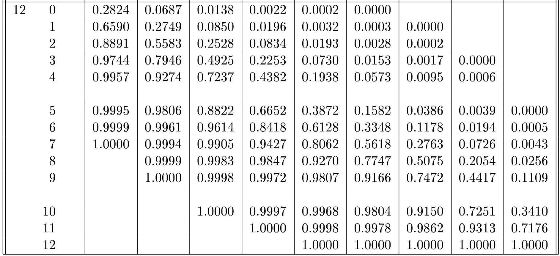
Figure 5.7: Tabulated c.d.f. values for the binomial distribution with \(n=12\) [source unknown].
The appropriate value \(\approx 0.9744\) can be found in the group corresponding to \(n=12\), in the row corresponding to \(x=3\), and in the column corresponding to \(p=0.1\).
The table can also be used to compute \[\begin{aligned} P(X=3)&=P(X\leq 3)-P(X\leq 2)\\&=0.9744-0.8891\approx 0.0853.\end{aligned}\]
An airline sells \(101\) tickets for a flight with \(100\) seats. Each passenger with a ticket is known to have a probability \(p=0.97\) of showing up for their flight. What is the probability of \(101\) passengers showing up (and the airline being caught overbooking)? Make appropriate assumptions. What if the airline sells 125 tickets?
Answer: let \(X\) be the number of passengers that show up. We want to compute \(P(X>100)\).
If all passengers show up independently of one another (no families or late bus?), we can model \(X\sim \mathcal{B}(101,0.97)\) and \[\begin{aligned} P(X&>100)=P(X=101)\\&=\binom{101}{101}(0.97)^{101}(0.03)^0\approx 0.046.\end{aligned}\] If the airline sells \(n=125\) tickets, we can model the situation with the binomial distribution \(\mathcal{B}(125,0.97)\), so that \[\begin{aligned} P(X&>100)=1-P(X\leq 100)\\&=1-\sum_{x=0}^{100}\binom{125}{x}(0.97)^x(0.03)^{125-x}.\end{aligned}\] This sum is harder to compute directly, but is very nearly \(1\) (try it in
R, say).Do these results match your intuition?
We can evaluate related probabilities in R via the base functions rbinom(), dbinom(), etc., whose parameters are n, size, and prob. You can probably guess what the next two block do.
[1] 5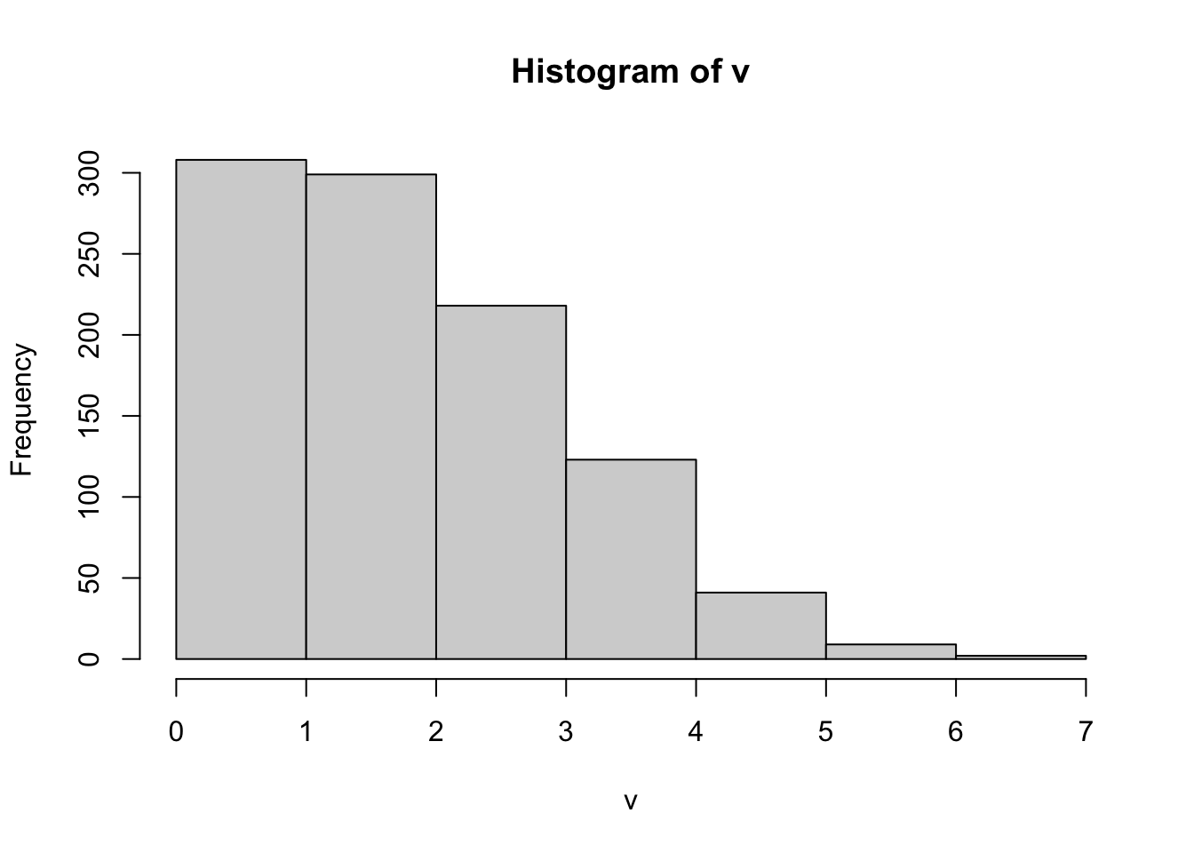
[1] 2.236
[1] 1.794098
# let's try another one
v<- rbinom(1000,size=19, prob=0.7)
mean(v)
var(v)
brks = min(v):max(v)
hist(v, breaks = brks)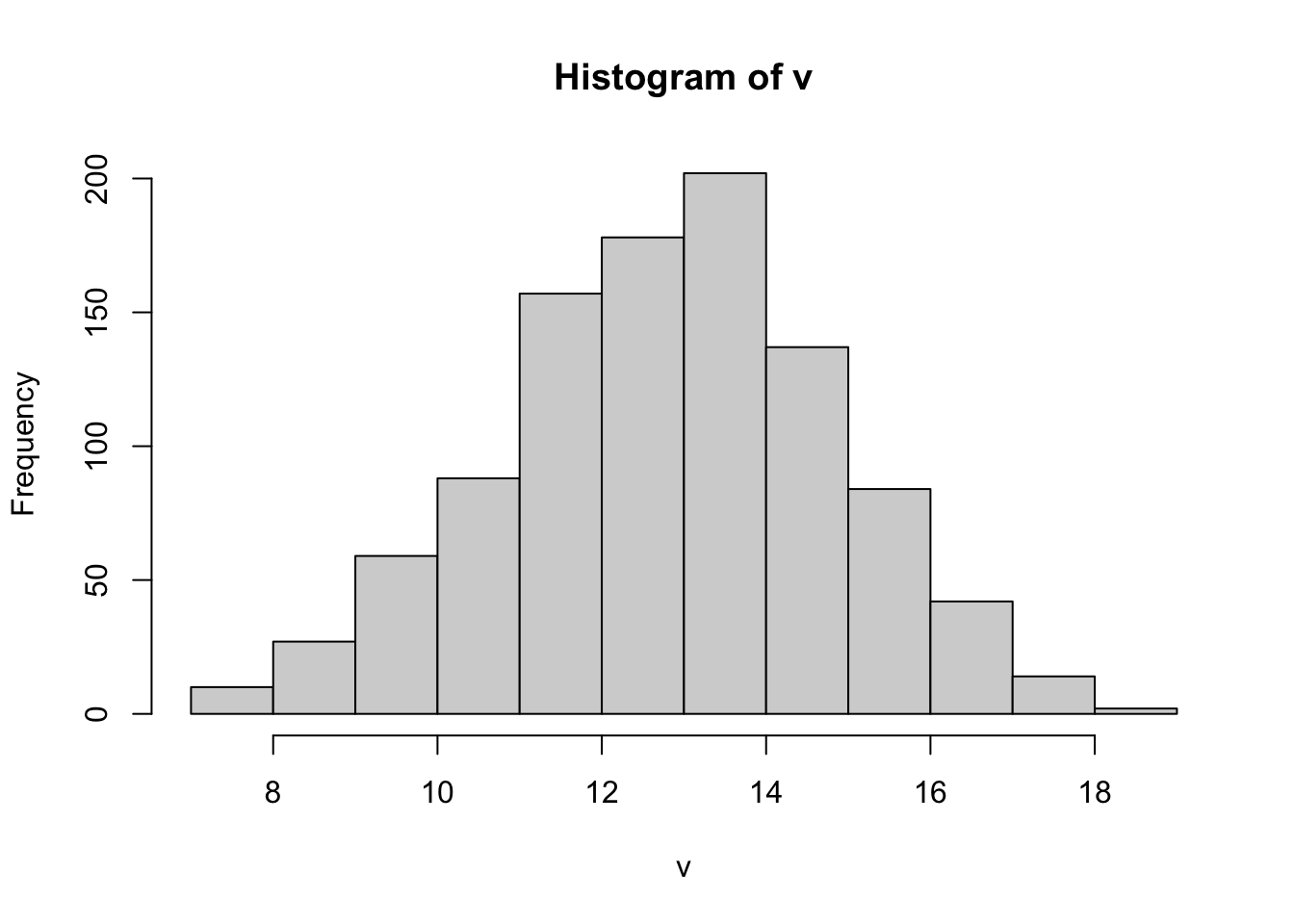
[1] 13.308
[1] 4.253389
5.2.4 Geometric Distributions
Now consider a sequence of Bernoulli trials, with probability \(p\) of success at each step. Let the geometric random variable \(X\) denote the number of steps before the first success occurs. The probability mass function is given by \[f(x)=P(X=x)=(1-p)^{x-1}p,\quad x=1,2,\ldots \] denoted \(X\sim \text{Geo}(p)\). For this random variable, we have \[\text{E}[X]=\frac{1}{p} \quad\mbox{and}\quad \text{Var}[X]=\frac{1-p}{p^2}.\] Examples:
A fair \(6-\)sided die is thrown until it shows a \(6\). What is the probability that \(5\) throws are required?
Answer: If \(5\) throws are required, we have to compute \(P(X=5)\), where \(X\) is geometric \(\text{Geo}(1/6)\): \[P(X=5)=(1-p)^{5-1}p=(5/6)^4(1/6)\approx 0.0804.\]
In the example above, how many throws would you expect to need?
Answer: \(\text{E}[X]=\frac{1}{1/6}=6\).
5.2.5 Negative Binomial Distribution
Consider now a sequence of Bernoulli trials, with probability \(p\) of success at each step. Let the negative binomial random variable \(X\) denote the number of steps before the \(r\)th success occurs.
The probability mass function is given by \[f(x)=P(X=x)=\binom{x-1}{r-1}(1-p)^{x-r}p^r,\quad x=r,r+1,\ldots\] which we denote by \(X\sim \text{NegBin}(p,r)\).
For this random variable, we have \[\text{E}[X]=\frac{r}{p} \quad\mbox{and}\quad \text{Var}[X]=\frac{r(1-p)}{p^2}.\]
Examples:
A fair \(6-\)sided die is thrown until it three \(6\)’s are rolled. What is the probability that \(5\) throws are required?
Answer: If \(5\) throws are required, we have to compute \(P(X=5)\), where \(X\) is geometric \(\text{NegBin}(1/6,3)\): \[\begin{aligned} P(X=5)&=\binom{5-1}{3-1}(1-p)^{5-3}p^3\\&=\binom{4}{2}(5/6)^2(1/6)^3\approx 0.0193. \end{aligned}\]
In the example above, how many throws would you expect to need?
Answer: \(\text{E}[X]=\frac{3}{1/6}=18\).
5.2.6 Poisson Distributions
Let us say we are counting the number of “changes” that occur in a continuous interval of time or space.9
We have a Poisson process with rate \(\lambda\), denoted by \(\mathcal{P}(\lambda)\), if:
the number of changes occurring in non-overlapping intervals are independent;
the probability of exactly one change in a short interval of length \(h\) is approximately \(\lambda h\), and
The probability of \(2+\) changes in a sufficiently short interval is essentially \(0\).
Assume that an experiment satisfies the above properties. Let \(X\) be the number of changes in a unit interval (this could be \(1\) day, or \(15\) minutes, or \(10\) years, etc.).
What is \(P(X=x)\), for \(x=0, 1, \ldots\)? We can get to the answer by first partition the unit interval into \(n\) disjoint sub-intervals of length \(1/n\). Then,
by the second condition, the probability of one change occurring in one of the sub-intervals is approximately \(\lambda/n\);
by the third condition, the probability of \(2+\) changes is \(\approx 0\), and
by the first condition, we have a sequence of \(n\) Bernoulli trials with probability \(p=\lambda/n\).
Therefore, \[\begin{aligned} f(x)&=P(X=x) \approx \frac{n!}{x!(n-x)!}\left(\frac{\lambda}{n}\right)^x\left(1-\frac{\lambda}{n}\right)^{n-x} \\ &=\frac{\lambda^x}{x!}\cdot\underbrace{\frac{n!}{(n-x)!}\cdot\frac{1}{n^x}}_{\text{term $1$}}\cdot\underbrace{\left(1-\frac{\lambda}{n}\right)^{n}}_{\text{term $2$}}\cdot\underbrace{\left(1-\frac{\lambda}{n}\right)^{-x}}_{\text{term $3$}}.\end{aligned}\] Letting \(n\to\infty\), we obtain \[\begin{aligned} P(X=x)&=\lim_{n\to\infty}\frac{\lambda^x}{x!}\cdot\underbrace{\frac{n!}{(n-x)!}\cdot\frac{1}{n^x}}_{\text{term $1$}}\cdot\underbrace{\left(1-\frac{\lambda}{n}\right)^{n}}_{\text{term $2$}}\cdot\underbrace{\left(1-\frac{\lambda}{n}\right)^{-x}}_{\text{term $3$}} \\ &=\frac{\lambda^x}{x!}\cdot 1 \cdot \exp(-\lambda)\cdot 1 = \frac{\lambda^xe^{-\lambda}}{x!}, \quad x=0, 1, \ldots \end{aligned}\] Let \(X\sim \mathcal{P}(\lambda)\). Then it can be shown that \[\text{E} [X]=\lambda \quad\mbox{and}\quad \text{Var} [X]=\lambda,\] that is, the mean and the variance of a Poisson random variable are identical.
We can compute related probabilities in R via the base functions rpois(), dpois(), etc., with required parameters n and lambda.
{r, fig.cap=NULL, rpois(1,lambda=13)
{r, fig.cap=NULL, u<-rpois(500,lambda=13) head(u) mean(u) var(u) hist(u)
Examples:
A traffic flow is typically modeled by a Poisson distribution. It is known that the traffic flowing through an intersection is \(6\) cars/minute, on average. What is the probability of no cars entering the intersection in a \(30\) second period?
Answer: \(6\) cars/min \(=\) \(3\) cars/\(30\) sec. Thus \(\lambda=3\), and we need to compute \[P(X=0)=\frac{3^0e^{-3}}{0!}=\frac{e^{-3}}{1}\approx 0.0498.\]
A hospital needs to schedule night shifts in the maternity ward. It is known that there are \(3000\) deliveries per year; if these happened randomly round the clock,[Is this a reasonable assumption?], we would expect \(1000\) deliveries between the hours of midnight and 8.00 a.m., a time when much of the staff is off-duty.
It is thus important to ensure that the night shift is sufficiently staffed to allow the maternity ward to cope with the workload on any particular night, or at least, on a high proportion of nights.
The average number of deliveries per night \[\lambda = 1000/365.25\approx 2.74.\] If the daily number \(X\) of night deliveries follows a Poisson process \(\mathcal{P}(\lambda)\), we can compute the probability of delivering \(x=0,1,2,\ldots\) babies on each night.
Some of the probabilities are:
For a Poisson distribution, the probability mass values \(f(x)\) can be obtained using
dpois()(for a general distribution, replace therin therxxxxx(...)random number generators byd:dxxxxx(...)).```{r, fig.cap=NULL, lambda = 2.74 # Poisson distribution parameter x=0:10 # in theory, goes up to infinity, but we’ve got to stop somewhere… y=dpois(x,lambda) # pmf z=ppois(x,lambda) # cmf
knitr::kable(data.frame(x,y,z))
5.2.6 pdf plot
plot(x,y, type=“h”, col=2, main=“Poisson PMF”, xlab=“x”, ylab=“f(x)=P(X=x)”)> points(x,y, col=2) abline(h=0, col=4)
5.2.6 cmf plot
plot(c(1,x),c(0,z), type=“s”, col=2, main=“Poisson CMF”, xlab=“x”, ylab=“F(x)=P(X<=x)”) abline(h=0:1, col=4) ```
If the maternity ward wants to prepare for the greatest possible traffic on \(80\%\) of the nights, how many deliveries should be expected?
Answer: we seek an \(x\) for which \[P(X\leq x-1)\leq 0.80\leq P(X\leq x).\]
# cmf  plot
lambda = 2.74 # Poisson distribution parameter
x=0:10 # in theory, goes up to infinity, but we've got to stop somewhere...
y=dpois(x,lambda) # pmf
z=ppois(x,lambda) # cmf
plot(c(1,x),c(0,z), type="s", col=2, main="Poisson CMF", xlab="x", ylab="F(x)=P(X<=x)")
abline(h=0:1, col=4)
abline(h=0.8, col=1)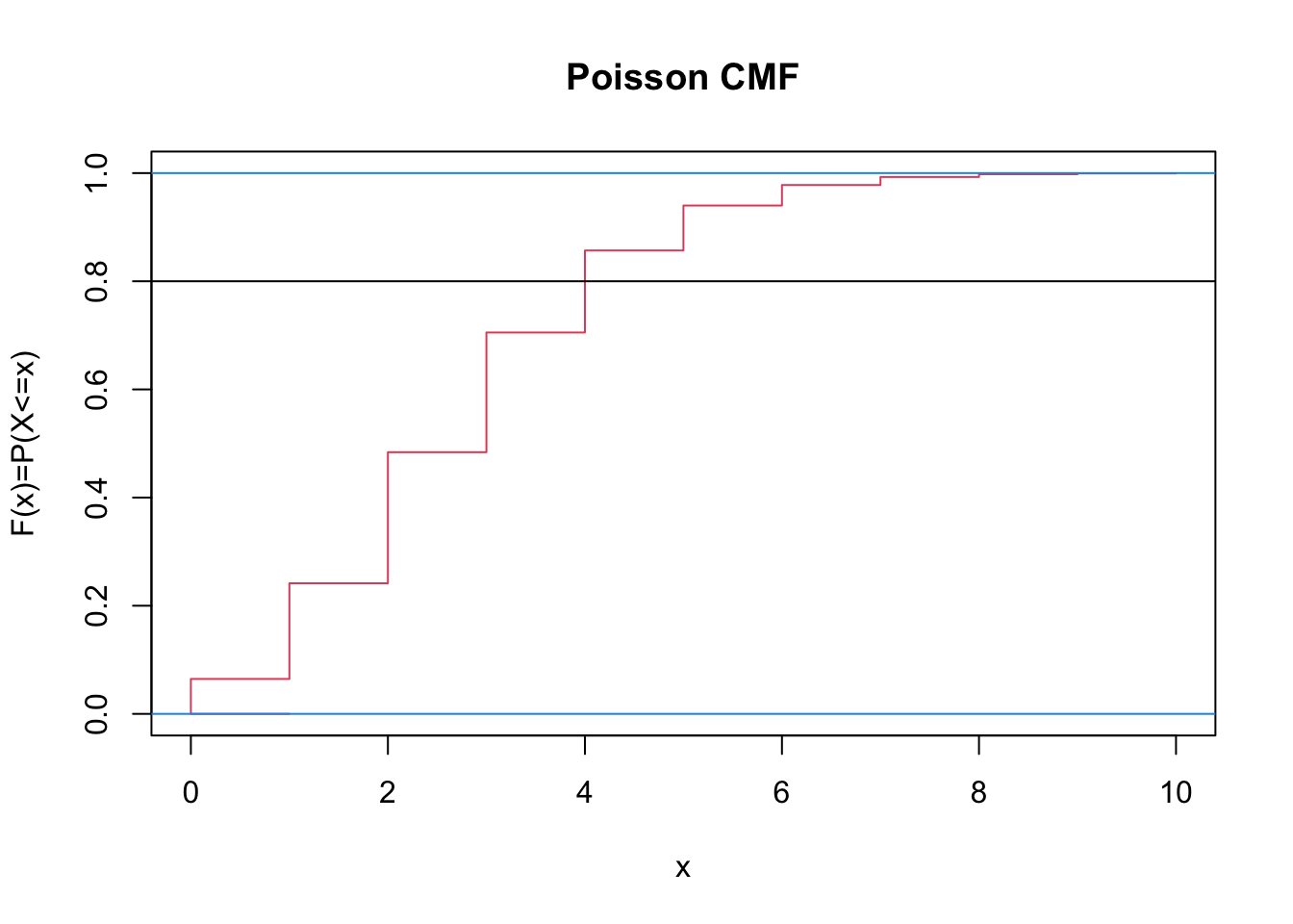
The \(y=0.8\) line crosses the CMF at \(x=4\); let’s evaluate \(F(3)=P(X\leq 3)\) and \(F(4)=P(X\leq 4)\) to confirm that \(F(3)\leq 0.8 \leq F(4)\).
[1] 0.7052548
[1] 0.8568984
It is indeed the case. Thus, if the hospital prepares for \(4\) deliveries a night, they will be ready for the worst on at least \(80\%\) of the nights (closer to \(85.7\%\), actually).
Note that this is different than asking how many deliveries are expected nightly (namely, \(\text{E}[X]=2.74\)).
On how many nights in the year would \(5\) or more deliveries be expected?
Answer: we need to evaluate \[\begin{aligned} 365.25\cdot P(X\ge 5)&=365.25 (1-P(X\le 4)). \end{aligned}\]
[1] 52.26785Thus, roughly \(14\%\) of the nights.
Over the course of one year, what is the greatest number of deliveries expected on any night?
Answer: we are looking for largest value of \(x\) for which \(365.25\cdot P(X=x)\geq 1\) (if \(365.25\cdot P(X=x)<1\), then the probability of that number of deliveries is too low to expect that we would ever see it during the year).
lambda=2.74

# initializing vector
nights=c()

# expected number of nights with each number of deliveries
for(j in 0:10){
  nights[j+1]=365.25*dpois(j,lambda)
}
rbind(0:10,nights)

# identify largest index
max(which(nights>1))-1
[,1] [,2] [,3] [,4] [,5] [,6] [,7] [,8] 0.00000 1.00000 2.00000 3.00000 4.00000 5.00000 6.00000 7.000000 nights 23.58432 64.62103 88.53082 80.85815 55.38783 30.35253 13.86099 5.425587 [,9] [,10] [,11] 8.000000 9.000000 10.0000000 nights 1.858264 0.565738 0.1550122 [1] 8Namely, \(x=8\). Indeed, for larger values of \(x\), \(365.25\cdot P(X=x)<1\).
[1] 1.858264
[1] 0.565738
5.2.7 Other Discrete Distributions
Wikipedia [9] lists other common discrete distributions:
the Rademacher distribution, which takes values \(1\) and \(-1\), each with probability \(1/2\);
the beta binomial distribution, which describes the number of successes in a series of independent Bernoulli experiments with heterogeneity in the success probability;
the discrete uniform distribution, where all elements of a finite set are equally likely (balanced coin, unbiased die, first card of a well-shuffled deck, etc.);
the hypergeometric distribution, which describes the number of successes in the first \(m\) of a series of \(n\) consecutive Bernoulli experiments, if the total number of successes is known;
the negative hypergeometric distribution, which describes the number of attempts needed to get the \(n\)th success in a series of Bernoulli experiments;
the Poisson binomial distribution, which describes the number of successes in a series of independent Bernoulli experiments with different success probabilities;
Benford’s Law, which describes the frequency of the first digit of many naturally occurring data.
Zipf’s Law, which describes the frequency of words in the English language;
the beta negative binomial distribution, which describes the number of failures needed to obtain \(r\) successes in a sequence of independent Bernoulli experiments;
etc.
5.3 Continuous Distributions
How do we approach probabilities where there there are uncountably infinitely many possible outcomes, such as one might encounter if \(X\) represents the height of an individual in the population, for instance (e.g., the outcomes reside in a continuous interval)? What is the probability that a randomly selected person is about \(6\) feet tall, say?
5.3.1 Continuous Random Variables
In the discrete case, the probability mass function \[f_X(x)=P(X=x)\] was the main object of interest. In the continuous case, the analogous role is played by the probability density function (p.d.f.), still denoted by \(f_X(x)\), but there is a major difference with discrete r.v.: \[f_X(x) \neq P(X=x).\] The (cumulative) distribution function (c.d.f.) of any such random variable \(X\) is also still defined by \[F_X(x)=P(X\leq x)\,,\] viewed as a function of a real variable \(x\); however \(P(X\leq x)\) is not simply computed by adding a few terms of the form \(P(X=x_i)\).
Note as well that \[\lim_{x\to -\infty}F_X(x)=0\quad\mbox{and}\quad\lim_{x\to +\infty}F_X(x)=1.\] We can describe the distribution of the random variable \(X\) via the following relationship between \(f_X(x)\) and \(F_X(x)\): \[f_X(x)=\frac{d}{dx}F_X(x);\] in the continuous case, probability theory is simply an application of calculus!
Area Under the Curve
For any \(a<b\), we have \[\left\{ X\leq b \right\} = \left\{ X\leq a \right\}\cup \left\{ a<X\leq b \right\},\] so that \[\begin{aligned} P\left( X\leq a \right)+P\left( a<X\leq b \right) &= P\left( X\leq b \right)\end{aligned}\] and thus \[\begin{aligned} P\left( a<X\leq b \right)&= P\left( X\leq b \right)- P\left( X\leq a \right)\\ &= F_X(b)-F_X(a)=\int_a^b f_X(x)\, dx\end{aligned}\]
Probability Density Function
The probability density function (p.d.f.) of a continuous random variable \(X\) is an integrable function \(f_X: X(\mathcal{S})\to \mathbb{R}\) such that:
\(f_X(x)>0\) for all \(x\in X(\mathcal{S})\) and \(\displaystyle{\lim_{x\to \pm \infty}f_X(x)=0}\);
\(\int_{\mathcal{S}}f_X(x)\, dx=1\);
for any event \(A=(a,b)=\{X|a<X<b\}\), \[P(A)=P((a,b))=\int_a^b f_X(x)\, dx,\]
and the cumulative distribution function (c.d.f.) \(F_X\) is given by \[F_X(x)=P(X\leq x)=\int_{-\infty}^xf_X(t)\, dt.\] Unlike discrete distributions, the absence or presence of endpoints does not affect the probability computations for continuous distributions: for any \(a,b\), \[P(a<X<b)=P(a\leq X<b)=P(a<X\leq b)=P(a\leq X\leq b),\] all taking the value \[F_X(b)-F_X(a)=\int_a^bf(x)\, dx.\] Furthermore, for any \(x\), \[P(x> X) = 1-P(X\leq x)=1-F_X(x)=1-\int_{-\infty}^xf_X(t)\, dt;\] and for any \(a\), \[P\left( X=a \right)= P\left( a\leq X\leq a \right)= \int_a^{a} f_X(x)\,dx=0.\] That last result explains why it is pointless to speak of the probability of a random variable taking on a specific value in the continuous case; rather, we are interested in ranges of values.
Examples
Assume that \(X\) has the following p.d.f.: \[f_X(x)=\begin{cases}0 & \text{if $x<0$} \\ x/2 & \text{if $0\leq x\leq 2$} \\ 0 & \text{if $x>2$}\end{cases}\] Note that \(\int_{0}^2f(x)\, dx =1.\) The corresponding c.d.f.is given by: \[\begin{aligned} F_X&(x)=P(X\leq x)=\int_{-\infty}^x f_X(t)\, dt \\ &=\begin{cases} 0 & \text{if $x<0$} \\ 1/2\cdot \int_{0}^x t\, dt = x^2/4 & \text{if $0<x<2$} \\ 1 & \text{if $x\geq 2$} \end{cases}\end{aligned}\]
The p.m.f. and the c.m.f. for this r.v. are shown in Figure 5.8.
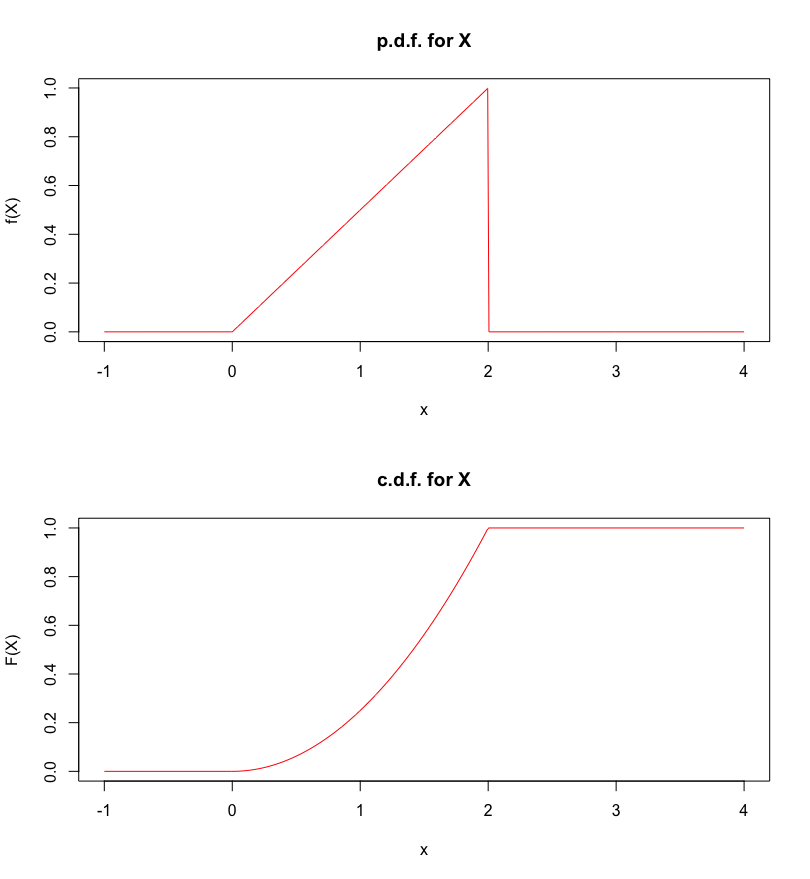
Figure 5.8: P.d.f. and c.d.f. for the r.v. \(X\) defined above.
What is the probability of the event \[A=\{X|0.5<X<1.5\}?\]
Answer: we need to evaluate \[\begin{aligned} P(A)&=P(0.5<X<1.5)=F_X(1.5)-F_X(0.5)\\ &=\frac{(1.5)^2}{4}-\frac{(0.5)^2}{4} =\frac{1}{2}. \end{aligned}\]
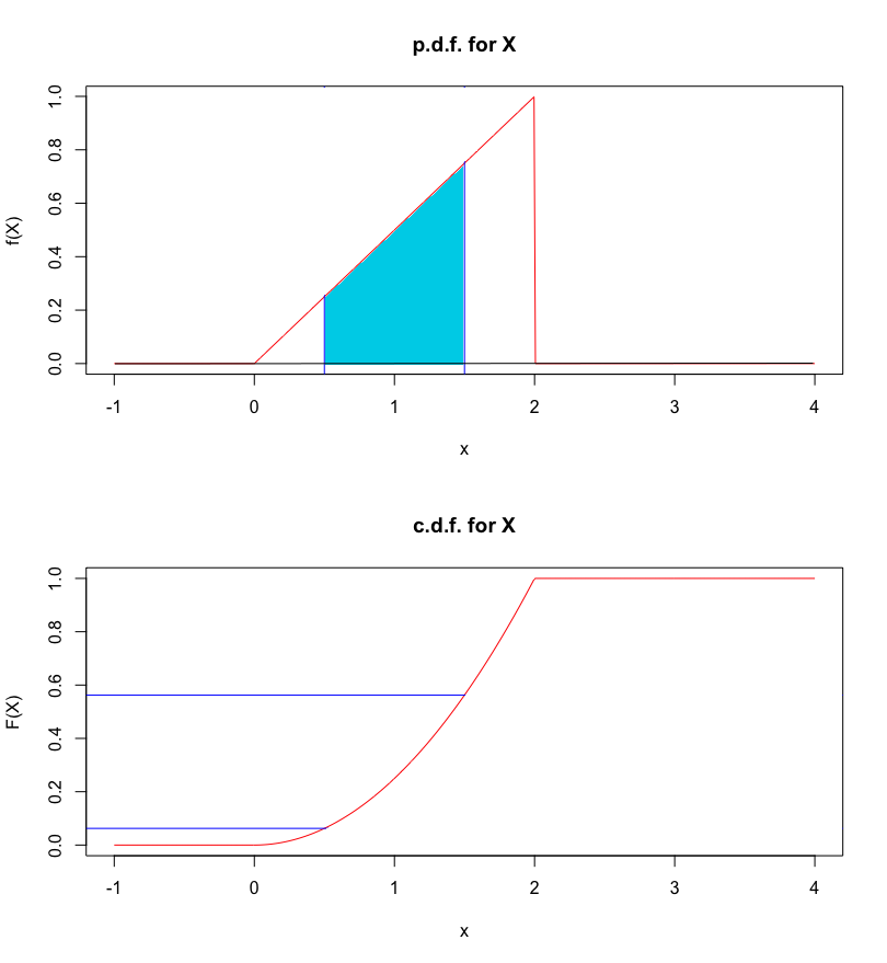
Figure 5.9: P.d.f. and c.d.f. for the r.v. \(X\) defined above, with appropriate region.
What is the probability of the event \(B=\{X|X=1\}\)?
Answer: we need to evaluate \[P(B) = P(X=1)=P(1\leq X\leq 1)=F_{X}(1)-F_X(1)=0.\] This is not unexpected: even though \(f_X(1)=0.5\neq 0\), \(P(X=1)=0\), as we saw earlier.
Assume that, for \(\lambda>0\), \(X\) has the following p.d.f.: \[f_X(x)=\begin{cases} \lambda\exp(-\lambda x) & \text{if $x\geq 0$}\\ 0&\text{if $x<0$} \end{cases}\] Verify that \(f_X\) is a p.d.f.for all \(\lambda>0\), and compute the probability that \(X>10.2\).
Answer: that \(f_X\) is a p.d.f.is obvious; the only work goes into showing that \[\begin{aligned} \int_{-\infty}^{\infty}&f(x)\, dx =\int_{0}^{\infty}\lambda\exp(-\lambda x)\, dx\\&=\lim_{b\to\infty}\int_{0}^{b}\lambda\exp(-\lambda x)\, dx\\&=\lim_{b\to\infty}\lambda \left[\frac{\exp(-\lambda x)}{-\lambda}\right]_0^b =\lim_{b\to\infty}\left[-\exp(-\lambda x)\right]_0^b\\ &=\lim_{b\to\infty}\left[-\exp(-\lambda b)+\exp(0)\right]=1.\end{aligned}\] The corresponding c.d.f.is given by: \[\begin{aligned} F_X(x;\lambda)&=P_{\lambda}(X\leq x)=\int_{-\infty}^{x}f_X(t)\, dt\\&=\begin{cases} 0 & \text{if $x<0$} \\ \lambda\int_0^x\exp(-\lambda t)\, dt & \text{if $x\geq 0$}\end{cases} \\ & = \begin{cases} 0 & \text{if $x<0$} \\ [-\exp(-\lambda t)]_0^x & \text{if $x\geq 0$} \end{cases} \\ &= \begin{cases} 0 & \text{if $x<0$} \\ 1-\exp(-\lambda x) & \text{if $x\geq 0$} \end{cases}\end{aligned}\] Then \[\begin{aligned} P_{\lambda}(X>10.2)&=1-F_X(10.2;\lambda)=1-[1-\exp(-10.2\lambda)]\\&=\exp(-10.2\lambda)\end{aligned}\] is a function of the distribution parameter \(\lambda\) itself:
\(\lambda\) \(P_{\lambda}(X>10.2)\) \(0.002\) \(0.9798\) \(0.02\) \(0.8155\) \(0.2\) \(0.1300\) \(2\) \(1.38 \times 10^{-9}\) \(20\) \(2.54 \times 10^{-89}\) \(200\) \(0\) (for all intents and purposes) For \(\lambda=0.2\), for instance, the p.d.f.and c.d.f.are:
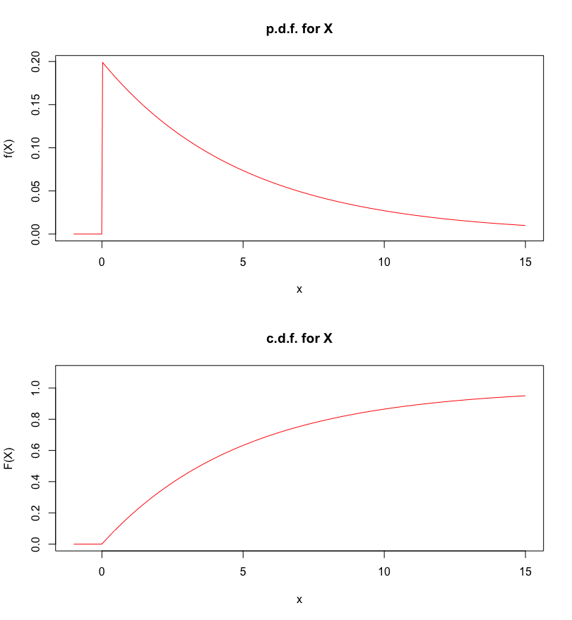
Figure 5.10: P.d.f. and c.d.f. for the r.v. \(X\) defined above, with \(\lambda=0.2\).
The probability that \(X>10.2\) is the area (to \(\infty\)) in blue, below.
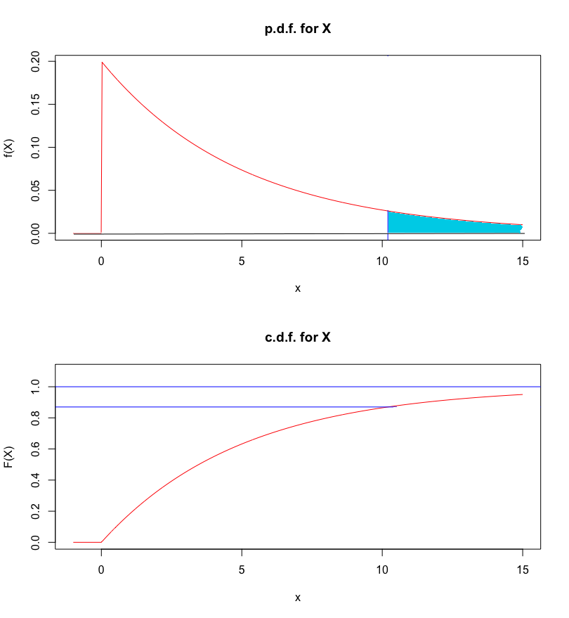
Figure 5.11: Probability of \(X>10.2\), for \(X\) defined above, with \(\lambda=0.2\).
For \(\lambda=2\), the probability is so small (\(1.38\times 10^{-9}\)) that it does not even appear in the p.d.f. (see below).
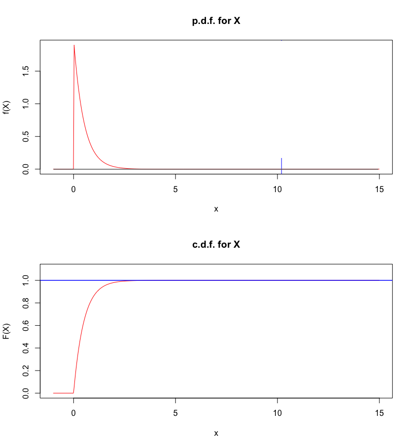
Figure 5.12: Probability of \(X>10.2\), for \(X\) defined above, with \(\lambda=2\).
Note that in all cases, the shape of the p.d.f.and the c.d.fare the same (the spike when \(\lambda=2\) is much higher than that when \(\lambda=0.2\) – why must that be the case?). This is not a general property of distributions, however, but a property of this specific family of distributions.
5.3.2 Expectation of a Continuous Random Variable
For a continuous random variable \(X\) with p.d.f.\(f_X(x)\), the expectation of \(X\) is defined as \[\text{E}[X]=\int_{-\infty}^\infty x f_X(x)\,dx\,.\] For any function \(h(X)\), we can also define \[\text{E}\left[ h(X) \right] = \int_{-\infty}^\infty h(x) f_X(x)\,dx\,.\]
Examples:
Find \(\text{E}[X]\) and \(\text{E}[X^2]\) in the first example, above.
Answer: we need to evaluate \[\begin{aligned} \text{E} [X]&=\int_{-\infty}^{\infty}xf_X(X)\, dx=\int_0^2xf_X(x)\,dx \\ &=\int_0^2\frac{x^2}{2}\, dx = \left[\frac{x^3}{6}\right]_{x=0}^{x=2}=\frac{4}{3};\\ \text{E}[X^2]&=\int_0^2\frac{x^3}{2}\, dx=2.\end{aligned}\]
Note that the expectation need not exist! Compute the expectation of the random variable \(X\) with p.d.f.\[f_X(x)=\frac{1}{\pi(1+x^2)}, \quad-\infty<x<\infty.\]
Answer: let’s verify that \(f_X(x)\) is indeed a p.d.f.: \[\begin{aligned} \int_{-\infty}^{\infty}f_X(x)\, dx&= \frac{1}{\pi}\int_{-\infty}^{\infty}\frac{1}{1+x^2}\, dx \\&= \frac{1}{\pi}[\arctan(x)]^{\infty}_{-\infty}=\frac{1}{\pi}\left[\frac{\pi}{2}+\frac{\pi}{2}\right]=1. \end{aligned}\]
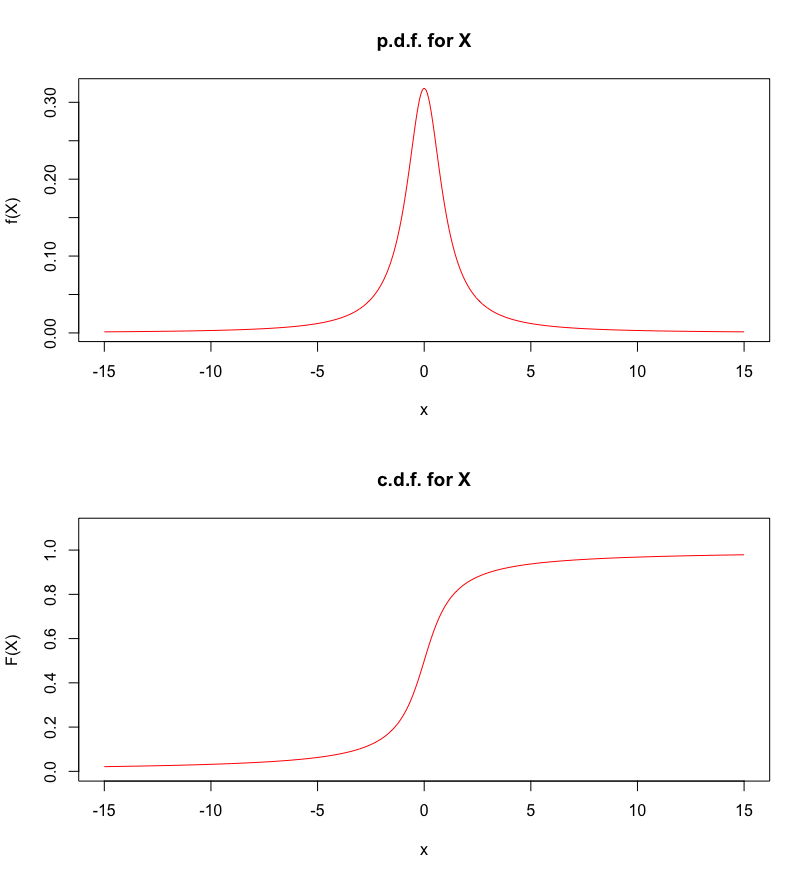
Figure 5.13: P.d.f. and c.d.f. for the Cauchy distribution.
We can also easily see that \[\begin{aligned} F_X(x)&=P(X\leq x)=\int_{-\infty}^xf_X(t)\, dt\\& =\frac{1}{\pi}\int_{-\infty}^x\frac{1}{1+t^2}\, dt=\frac{1}{\pi}\arctan(x)+\frac{1}{2}.\end{aligned}\] For instance, \(P(X\leq 3)=\frac{1}{\pi}\arctan(3)+\frac{1}{2}\), say.
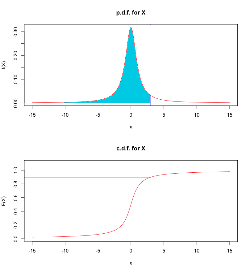
Figure 5.14: P.d.f. and c.d.f. for the Cauchy distribution, with area under the curve.
The expectation of \(X\) is \[\begin{aligned} \text{E}[X]&=\int_{-\infty}^{\infty}xf_X(x)\, dx = \int_{-\infty}^{\infty}\frac{x}{\pi(1+x^2)}\, dx.\end{aligned}\] If this improper integral exists, then it needs to be equal both to \[\underbrace{\int_{-\infty}^0\frac{x}{\pi(1+x^2)}\, dx + \int_0^{\infty}\frac{x}{\pi(1+x^2)}\, dx}_{\text{candidate $1$}}\] and to the Cauchy principal value \[\underbrace{\lim_{a\to\infty}\int_{-a}^a\frac{x}{\pi(1+x^2)}\, dx}_{\text{candidate $2$}}.\] But it is straightforward to find an antiderivative of \(\frac{x}{\pi(1+x^2)}.\) Set \(u=1+x^2\). Then \(du=2xdx\) and \(xdx=\frac{du}{2}\), and we obtain \[\int \frac{x}{\pi(1+x^2)}\, dx=\frac{1}{2\pi}\int u\, du=\frac{1}{2\pi}\ln|u|=\frac{1}{2\pi}\ln(1+x^2).\] Then the candidate \(2\) integral reduces to \[\begin{aligned} \lim_{a\to\infty}\left[\frac{\ln(1+x^2)}{2\pi}\right]_{-a}^a&=\lim_{a\to\infty}\left[\frac{\ln(1+a^2)}{2\pi}-\frac{\ln(1+(-a)^2)}{2\pi}\right] \\ &=\lim_{a\to\infty}0=0;\end{aligned}\] while the candidate \(1\) integral reduces to \[\left[\frac{\ln(1+x^2)}{2\pi}\right]^0_{-\infty}+\left[\frac{\ln(1+x^2)}{2\pi}\right]^{\infty}_0 =0-(\infty)+\infty-0=\infty-\infty\] which is undefined. Thus \(\text{E}[X]\) cannot not exist, as it would have to be both equal to \(0\) and be undefined simultaneously.
Mean and Variance
In a similar way to the discrete case, the mean of \(X\) is defined to be \(\text{E}[X]\), and the \(\textbf{variance}\) and standard deviation of \(X\) are, as before, \[\begin{aligned} \text{Var}[X]&\stackrel{\text{def}}= \text{E}\left[( X-\text{E}[X])^2 \right] =\text{E}[X^2]- \text{E}^2[X]\,, \\ \text{SD}[X]&=\sqrt{\text{Var}[X]}\,.\end{aligned}\] As in the discrete case, if \(X,Y\) are continuous random variables, and \(a,b\in\mathbb{R}\), then \[\begin{aligned} \text{E}[aY+bX]&= a\text{E}[Y]+b\text{E}[X]\\ \text{Var}[ a+bX ]&= b^2\text{Var}[X]\\ \text{SD}[ a+bX ]&=|b|\text{SD}[X]\end{aligned}\] The interpretations of the mean as a measure of centrality and of the variance as a measure of dispersion are unchanged in the continuous case.
For the time being, however, we cannot easily compute the variance of a sum \(X+Y\), unless \(X\) and \(Y\) are independent random variables, in which case \[\text{Var}[X+Y]= \text{Var}[X]+\text{Var}[Y].\]
5.3.3 Normal Distributions
A very important example of a continuous distribution is that provided by the special probability distribution function \[\phi(z)=\frac1{\sqrt{2\pi}}e^{-z^2/2}\,.\] The corresponding cumulative distribution function is denoted by \[\Phi(z)=P(Z\leq z)=\int_{-\infty}^z \phi(t)\,dt\,.\] A random variable \(Z\) with this c.d.f.is said to have a standard normal distribution, denoted by \(Z\sim\mathcal N(0,1)\).
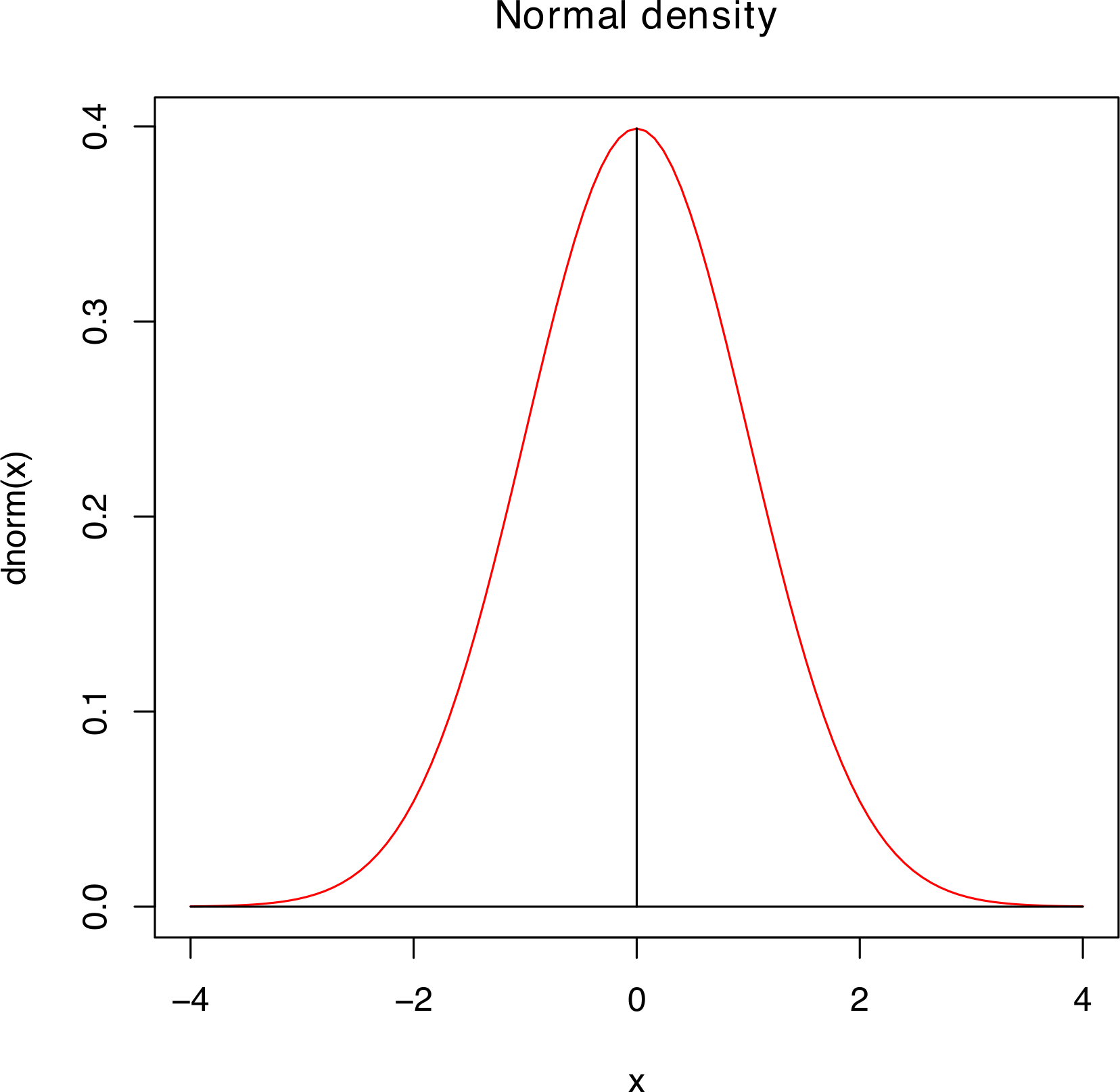
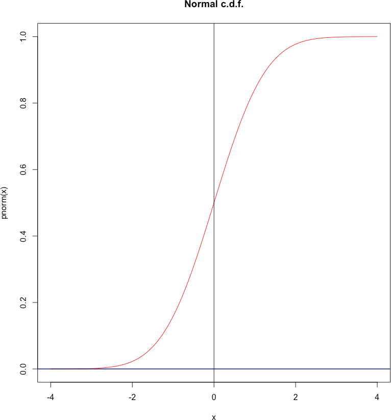
Figure 5.15: P.d.f. and c.d.f. for the standard normal distribution.
Standard Normal Random Variable
The expectation and variance of \(Z\sim\mathcal{N}(0,1)\) are \[\begin{aligned} \text{E}[Z]&= \int_{-\infty}^\infty z\, \phi(z)\, dz = \int_{-\infty}^{\infty}z\,\frac1{\sqrt{2\pi}} e^{-\frac12 z^2}\,dz =0, \\ \text{Var}[Z]&=\int_{-\infty}^{\infty}z^2\, \phi(z)\, dz = 1, \\ \text{SD}[Z]&=\sqrt{\text{Var}[Z]}=\sqrt{1}=1.\end{aligned}\] Other quantities of interest include: \[\begin{aligned} \Phi(0)&=P(Z\leq 0)=\frac{1}{2},\quad \Phi(-\infty)=0,\quad \Phi(\infty)=1,\\ \Phi(1)&=P(Z\leq 1)\approx 0.8413, \quad \text{etc.}\end{aligned}\]
Normal Random Variables
Let \(\sigma>0\) and \(\mu \in \mathbb{R}\).
If \(Z\sim\mathcal{N}(0,1)\) and \(X=\mu+\sigma Z\), then \[\frac{X-\mu}\sigma = Z \sim\mathcal{N}(0,1).\] Thus, the c.d.f.of \(X\) is given by \[\begin{aligned} F_X(x)&=P( X\leq x ) \\&= P( \mu+\sigma Z\leq x ) =P\left( Z\leq \frac{x-\mu}\sigma \right)\\&= \Phi\left( \frac{x-\mu}\sigma \right)\,;\end{aligned}\] its p.d.f. must then be \[\begin{aligned} f_X(x)&=\frac d{dx}F_X(x) \\&= \frac d{dx} \Phi\left( \frac{x-\mu}\sigma \right)\\ &= \frac1\sigma\, \phi\left( \frac{x-\mu}\sigma \right).\end{aligned}\] Any random variable \(X\) with this c.d.f./p.d.f.satisfies \[\begin{aligned} \text{E}[X]&=\mu+\sigma\text{E}[Z]=\mu,\\ \text{Var}[X]&=\sigma^2\text{Var}[Z]=\sigma^2, \\ \text{SD}[X]&=\sigma\end{aligned}\] and is said to be normal with mean \(\mu\) and variance \({\sigma^2}\), denoted by \(X\sim\mathcal{N}(\mu,\sigma^2)\).
As it happens, every general normal \(X\) can be obtained by a linear transformation of the standard normal \(Z\). Traditionally, probability computations for normal distributions are done with tables which compile values of the standard normal distribution c.d.f., such as the one found in [10] (see for a preview). With the advent of freely-available statistical software, the need for tabulated values had decreased.10
In R, the standard normal c.d.f. \(F_Z(z)=P(Z\leq z)\) can be computed
with the function pnorm(z) – for instance, pnorm(0)=0.5. (In the
example below, whenever \(P(Z\leq a)\) is evaluated for some \(a\), the
value is found either by consulting a table or using pnorm.)
Examples
Let \(Z\) represent the standard normal random variable. Then:
\(P(Z\le 0.5)=0.6915\)
\(P(Z<-0.3)=0.3821\)
\(P(Z>0.5)=1-P(Z\le 0.5)=1-0.6915=0.3085\)
\(P(0.1<Z<0.3)=P(Z<0.3)-P(Z<0.1)=0.6179-0.5398=0.0781\)
\(P(-1.2<Z<0.3)=P(Z<0.3)-P(Z<-1.2)=0.5028\)
Suppose that the waiting time (in minutes) in a coffee shop at 9am is normally distributed with mean \(5\) and standard deviation \(0.5\).11 What is the probability that the waiting time for a customer is at most \(6\) minutes?
Answer: let \(X\) denote the waiting time.
Then \(X\sim\mathcal{N}(5,0.5^2)\) and the standardised random variable is a standard normal: \[Z=\frac{X-5}{0.5} \sim\mathcal{N}(0,1)\,.\] The desired probability is \[\begin{aligned} P\left(X\leq6 \right) &= P\left( \frac{X-5}{0.5}\leq \frac{6-5}{0.5} \right)\\ & = P\left(Z\le \frac{6-5}{0.5} \right)= \Phi\left( \frac{6-5}{0.5} \right)\\&=\Phi(2)=P(Z\leq 2)\approx 0.9772 .\end{aligned}\]
Suppose that bottles of beer are filled in such a way that the actual volume of the liquid content (in mL) varies randomly according to a normal distribution with \(\mu=376.1\) and \(\sigma=0.4\).12 What is the probability that the volume in any randomly selected bottle is less than \(375\)mL?
Answer: let \(X\) denote the volume of the liquid in the bottle. Then \[\begin{aligned} X\sim\mathcal{N}(376.1,0.4^2)\implies Z=\frac{X-376.1}{0.4}\sim\mathcal{N}(0,1)\,.\end{aligned}\] The desired probability is thus \[\begin{aligned} P\left( X<375 \right) &= P\left( \frac{X-376.1}{0.4}<\frac{375-376.1}{0.4} \right) \\ &=P\left( Z<\frac{-1.1}{0.4} \right)\\&=P(Z\leq -2.75)=\Phi\left( -2.75 \right)\approx 0.003\,.\end{aligned}\]
If \(Z\sim\mathcal{N}(0,1)\), for which values \(a\), \(b\) and \(c\) do:
\(P(Z\leq a)=0.95\);
\(P(|Z|\le b)=P(-b\leq Z\leq b)=0.99\);
\(P(|Z|\geq c)=0.01\).
Answer:
From the table (or
R) we see that \[P(Z\leq 1.64)\approx 0.9495,\ P(Z\leq 1.65)\approx 0.9505\,.\] Clearly we must have \(1.64<a<1.65\); a linear interpolation provides a decent guess at \(a\approx1.645\).13Note that \[P\left( -b\leq Z\leq b \right)=P(Z\leq b)-P(Z<-b)\] However the p.d.f.\(\phi(z)\) is symmetric about \(z=0\), which means that \[P(Z<-b)=P(Z>b)=1-P(Z\leq b),\] and so that \[\begin{aligned} P\left( -b\leq Z\leq b \right)&=P(Z\leq b)-\left[ 1-P(Z\leq b) \right]\\& =2P(Z\leq b)-1\end{aligned}\] In the question, \(P(-b\le Z \le b)=0.99\), so that \[\begin{aligned} 2P(Z\le b)-1=0.99\implies \ P(Z\leq b)=\frac{1+0.99}2 = 0.995\,.\end{aligned}\] Consulting the table we see that \[P(Z\leq 2.57)\approx 0.9949,\ P(Z\leq 2.58)\approx 0.9951;\] a linear interpolation suggests that \(b\approx2.575\).
Note that \(\left\{ |Z|\geq c \right\}=\left\{ |Z|<c \right\}^c\), so we need to find \(c\) such that \[\begin{aligned} P\left(|Z|<c \right)=1-P\left( |Z|\geq c \right) = 0.99.\end{aligned}\] But this is equivalent to \[\begin{aligned} P\left( -c<Z<c \right)=P(-c\leq Z\leq c)=0.99\end{aligned}\] as \(|x|<y \Leftrightarrow -y<x<y\), and \(P(Z=c)=0\) for all \(c\). This problem was solved in part b); set \(c\approx 2.575\).
Normally distributed numbers can be generated by rnorm() in R, which accepts three parameters: n, mean, and sd. The default parameter values are mean=0 and sd=1.
[1] 1.606623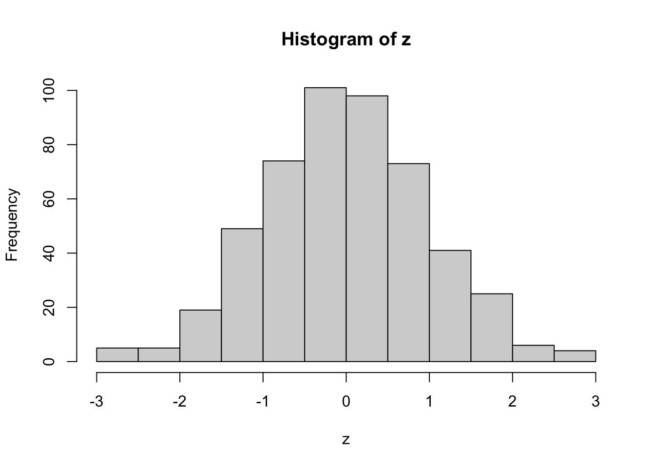
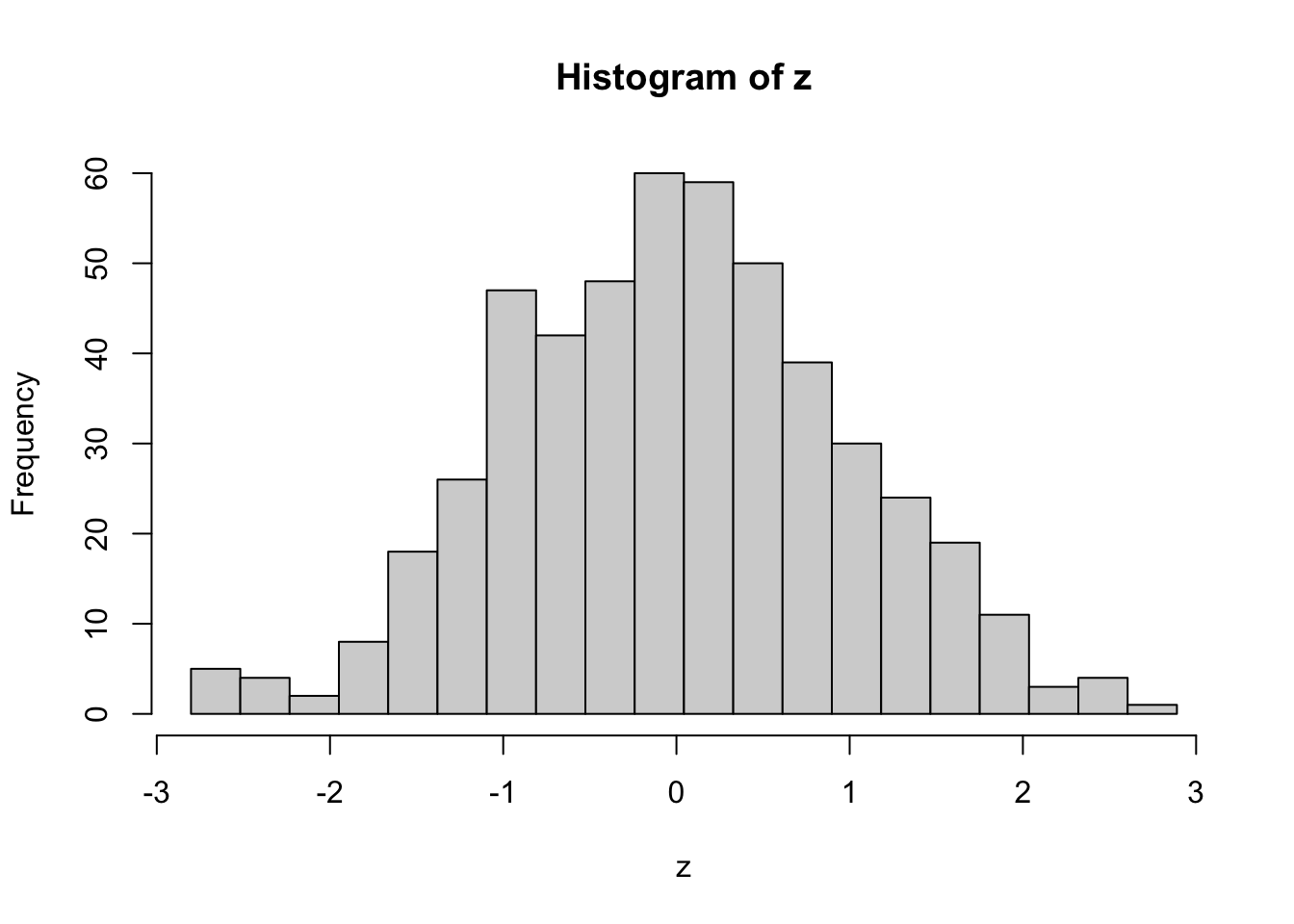
For normal distributions with specific mean \(\mu\) and standard deviation \(\sigma\), we need to modify the call to rnorm().
w<-rnorm(5000, sd=3, mean=-2)
mean(w)
sd(w)
brks = seq(min(w),max(w),(max(w)-min(w))/50)
hist(w, breaks = brks)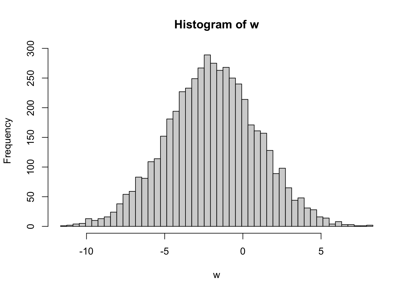
[1] -1.946337
[1] 2.911727
5.3.4 Exponential Distributions
Assume that cars arrive according to a Poisson process with rate \(\lambda\), that is, the number of cars arriving within a fixed unit time period is a Poisson random variable with parameter \(\lambda\).
Over a period of time \(x\), we would then expect the number of arrivals \(N\) to follow a Poisson process with parameter \(\lambda x\). Let \(X\) be the wait time to the first car arrival. Then \[P(X>x)=1-P(X\leq x)=P(N=0)=\exp(-\lambda x).\] We say that \(X\) follows an exponential distribution \(\text{Exp}(\lambda)\): \[\begin{aligned} F_X(x)&=\begin{cases} 0 & \text{for $x<0$} \\ 1-e^{-\lambda x} & \text{for $0\leq x$} \end{cases} \\ f_X(x)&=\begin{cases} 0 & \text{for $x<0$} \\ \lambda e^{-\lambda x} & \text{for $0\leq x$} \end{cases} \end{aligned}\] Note that \(f_X(x)=F'_X(x)\) for all \(x\).
If \(X\sim\text{Exp}(4)\), then \(P(X< 0.5)=F_X(0.5)=1-e^{-4(0.5)}\approx 0.865\) is the area of the shaded region in Figure 5.16, below.
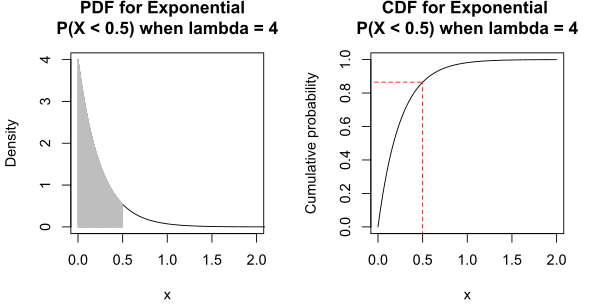
Figure 5.16: P.d.f. and c.d.f. for the exponential distribution. with parameter \(\lambda=4\) [source unknown].
Properties
If \(X\sim\text{Exp}(\lambda)\), then
\(\mu=\text{E} [X]=1/\lambda\), since \[\begin{aligned} \mu&=\int_{0}^{\infty}x\lambda e^{-\lambda x}\, dx=\left[-\frac{\lambda x+1}{\lambda}e^{-\lambda x}\right]_{0}^{\infty} \\ &=\left[0+\frac{\lambda(0)+1}{\lambda}e^{-0}\right]\\&=\frac{1}{\lambda}; \end{aligned}\]
\(\sigma^2=\text{Var} [X]=1/\lambda^2\), since \[\begin{aligned} \sigma^2&=\int_{0}^{\infty}\left(x-\text{E}[X]\right)^2\lambda e^{-\lambda x}\, dx\\&=\int_{0}^{\infty}\left(x-\frac{1}{\lambda}\right)^2\lambda e^{-\lambda x}\, dx\\&=\left[-\frac{\lambda^2 x^2+1}{\lambda^2}e^{-\lambda x}\right]_{0}^{\infty} \\ &=\left[0+\frac{\lambda^2(0)^2+1}{\lambda^2}e^{-0}\right]\\&=\frac{1}{\lambda^2}; \end{aligned}\]
and \(P(X>s+t\mid X>t)=P(X>s),\) for all \(s,t>0\), since \[\begin{aligned} P(X>s+t&\mid X>t)= \frac{P(X>s+t \text{ and } X>t)}{P(X>t)} \\&=\frac{P(X>s+t)}{P(X>t)}=\frac{1-F_X(s+t)}{1-F_X(t)} \\&=\frac{\exp(-\lambda (s+t))}{\exp(-\lambda t)}\\& =\exp(-\lambda s)=P(X>s)\end{aligned}\] (we say that exponential distributions are memoryless).
In a sense, \(\text{Exp}(\lambda)\) is the continuous analogue to the geometric distribution \(\text{Geo}(p)\).
Example: the lifetime of a certain type of light bulb follows an exponential distribution whose mean is \(100\) hours (i.e. \(\lambda=1/100\)).
What is the probability that a light bulb will last at least \(100\) hours?
Answer: Since \(X\sim \text{Exp}(1/100)\), we have \[P(X>100)=1-P(X\le 100)=\exp(-100/100)\approx 0.37.\]
Given that a light bulb has already been burning for \(100\) hours, what is the probability that it will last at least \(100\) hours more?
Answer: we seek \(P(X>200\mid X>100)\). By the memory-less property, \[P(X>200\mid X>100)=P(X>200-100)=P(X>100)\approx 0.37.\]
The manufacturer wants to guarantee that their light bulbs will last at least \(t\) hours. What should \(t\) be in order to ensure that \(90\%\) of the light bulbs will last longer than \(t\) hours?
Answer: we need to find \(t\) such that \(P(X>t)=0.9\). In other words, we are looking for \(t\) such that \[0.9=P(X>t)=1-P(X\leq t)=1-F_X(t)=e^{-0.01t},\] that is, \[\ln 0.9 = -0.01t \Longrightarrow t=-100\ln 0.9 \approx 10.5 \text{ hours}.\]
Exponentially distributed numbers are generated by rexp() in R, with required parameters n and rate.
[1] 0.006745894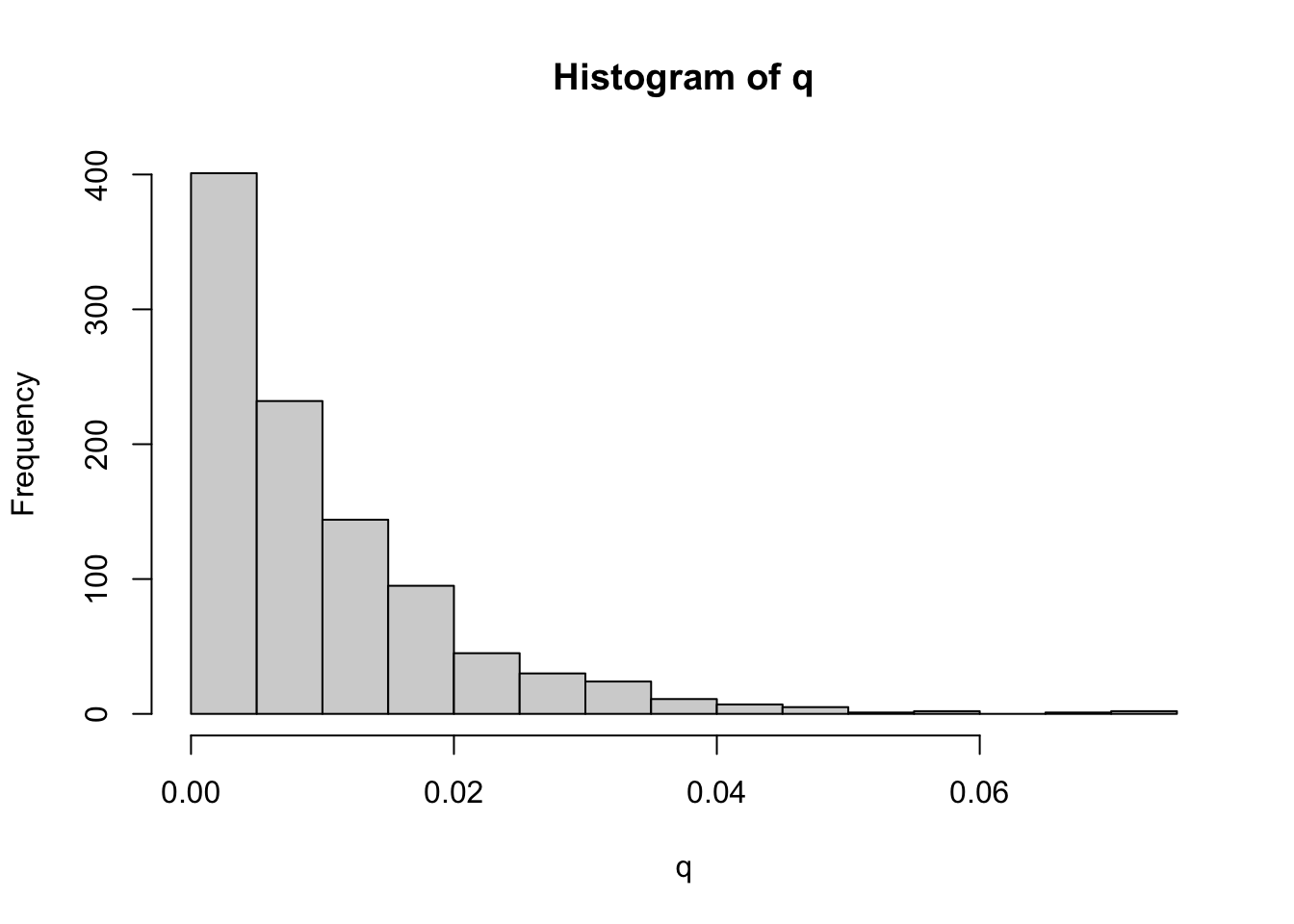
[1] 0.009958737
[1] 0.0001003328
5.3.5 Gamma Distributions
Assume that cars arrive according to a Poisson process with rate \(\lambda\). Recall that if \(X\) is the time to the first car arrival, then \(X\sim \text{Exp}(\lambda)\).
If \(Y\) is the wait time to the \(r\)th arrival, then \(Y\) follows a Gamma distribution with parameters \(\lambda\) and \(r\), denoted \(Y\sim \Gamma(\lambda,r)\), for which the p.d.f.is \[f_Y(y)=\begin{cases} 0 & \text{for $y<0$} \\ \frac{y^{r-1}}{(r-1)!}\lambda^r e^{- \lambda y } & \text{for $y\geq 0$} \end{cases}\] The c.d.f.\(F_Y(y)\) exists (it is the area under \(f_Y\) from \(0\) to \(y\)), but it cannot be expressed with elementary functions.
We can show that \[\mu=\text{E}[Y]=\frac{r}{\lambda}\quad\mbox{and}\quad\sigma^2=\text{Var}[Y]=\frac{r}{\lambda^2}.\]
Examples
Suppose that an average of \(30\) customers per hour arrive at a shop in accordance with a Poisson process, that is to say, \(\lambda=1/2\) customers arrive on average every minute. What is the probability that the shopkeeper will wait more than \(5\) minutes before both of the first two customers arrive?
Answer: let \(Y\) denote the wait time in minutes until the second customer arrives. Then \(Y\sim \Gamma(1/2,2)\) and \[\begin{aligned} P(Y>5)&=\int_{5}^{\infty}\frac{y^{2-1}}{(2-1)!}(1/2)^2e^{-y/2}\, dy\\&=\int_5^{\infty}\frac{ye^{-y/2}}{4}\, dy \\ &=\frac{1}{4}\left[-2ye^{-y/2}-4e^{-y/2}\right]_{5}^{\infty}\\&=\frac{7}{2}e^{-5/2}\approx 0.287.\end{aligned}\]
Telephone calls arrive at a switchboard at a mean rate of \(\lambda=2\) per minute, according to a Poisson process. Let \(Y\) be the waiting time until the \(5\)th call arrives. What is the p.d.f., the mean, and the variance of \(Y\)?
Answer: we have \[\begin{aligned} f_Y(y)&=\frac{2^5y^4}{4!}e^{-2y}, \text{ for $0\leq y<\infty$},\\ \quad \text{E}[Y]&=\frac{5}{2}, \quad \text{Var}[Y]=\frac{5}{4}.\end{aligned}\]
The Gamma distribution can be extended to cases where \(r>0\) is not an integer by replacing \((r-1)!\) by \[\Gamma(r)=\int_{0}^{\infty}t^{r-1}e^{-t}\, dt.\] The exponential and the \(\chi^2\) distributions (we will discuss the latter later) are special cases of the Gamma distribution: \(\text{Exp}(\lambda)=\Gamma(\lambda,1)\) and \(\chi^2(r)=\Gamma(1/2,r)\).
Gamma distributed numbers are generated by rgamma(), with required parameters n, shape, and scale.
[1] 0.9041355
[1] 0.6642976
[1] 0.2154044
5.3.6 Normal Approximation of the Binomial Distribution
If \(X\sim\mathcal{B}(n,p)\) then we may interpret \(X\) as a sum of independent and identically distributed random variables \[X=I_1+I_2+\cdots+I_n\ \text{ where each }\ I_i\sim\mathcal{B}(1,p)\,.\] Thus, according to the Central Limit Theorem (we will have more to say on the topic in a future section), for large \(n\) we have \[\frac{X-np}{\sqrt{np(1-p)}}\stackrel{\text{approx}}\sim\mathcal{N}(0,1)\,;\] for large \(n\) if \(X\stackrel{\text{exact}}\sim\mathcal{B}(n,p)\) then \(X\stackrel{\text{approx}}\sim\mathcal{N}(np,np(1-p))\).
Normal Approximation with Continuity Correction
When \(X\sim \mathcal{B}(n,p)\), we know that \(\text{E}[X]=np\) and \(\text{Var}[X]=np(1-p)\). If \(n\) is large, we may approximate \(X\) by a normal random variable in the following way: \[P(X\le x)=P(X<x+0.5)=P\left(Z<\frac{x-np+0.5}{\sqrt{np(1-p)}}\right)\] and \[P(X\ge x)=P(X>x-0.5)=P\left(Z>\frac{x-np-0.5}{\sqrt{np(1-p)}}\right).\] The continuity correction terms are the corresponding \(\pm 0.5\) in the expressions (they are required).
Example: suppose \(X\sim\mathcal{B}(36,0.5)\). Provide a normal approximation to the probability \(P(X\leq 12)\).14
Answer: the expectation and the variance of a binomial r.v.are known: \[\text{E}[X]=36(0.5)=18\quad\mbox{and}\quad \text{Var}[X]=36(0.5)(1-0.5) =9,\] and so \[\begin{aligned} P(X\leq12) &= P\left( \frac{X-18}{3}\leq\frac{12-18+0.5}{3}\right)\\ &\stackrel{\text{norm.approx'n}}\approx\Phi(-1.83) \stackrel{\text{table}}\approx0.033\,.\end{aligned}\]
Computing Binomial Probabilities
There are thus at least four ways of computing (or approximating) binomial probabilities:
using the exact formula – if \(X\sim\mathcal{B}(n,p)\) then for each \(x=0,1,\ldots,n\), \(P(X=x)=\binom nxp^x(1-p)^{n-x}\);
using tables: if \(n\leq15\) and \(p\) is one of \(0.1,\ldots,0.9\), then the corresponding c.d.f.can be found in many textbook (we must first express the desired probability in terms of the c.d.f. \(P(X\leq x)\)), such as in \[\begin{aligned} P(X<3)&=P(X\leq2); \\ P(X=7)&=P(X\leq7)-P(X\leq6) \,;\\ P(X>7)&=1-P(X\leq 7);\\ P(X\geq5)&=1-P(X\leq4),\, \text{ etc.}\end{aligned}\]
using statistical software (
pbinom()inR, say), andusing the normal approximation when \(np\) and \(n(1-p)\) are both \(\geq5\): \[P(X\leq x)\approx \Phi\left( \frac{x+0.5-np}{\sqrt{np(1-p)}} \right)\] \[P(X\ge x)\approx 1-\Phi\left( \frac{x-0.5-np}{\sqrt{np(1-p)}} \right).\]
5.3.7 Other Continuous Distributions
Other common continuous distributions are listed in [9]:
the Beta distribution, a family of 2-parameter distributions with one mode and which is useful to estimate success probabilities (special cases: uniform, arcsine, PERT distributions);
the logit-normal distribution on \((0,1)\), which is used to model proportions;
the Kumaraswamy distribution, which is used in simulations in lieu of the Beta distribution (as it has a closed form c.d.f.);
the triangular distribution, which is typically used as a subjective description of a population for which there is only limited sample data (it is based on a knowledge of the minimum and maximum and a guess of the mode);
the chi-squared distribution, which is the sum of the squares of \(n\) independent normal random variables, is used in goodness-of-fit tests in statistics;
the \(F-\)distribution, which is the ratio of two chi-squared random variables, used in the analysis of variance;
the Erlang distribution is the distribution of the sum of \(k\) independent and identically distributed exponential random variables, and it is used in queueing models (it is a special case of the Gammma distribution);
the Pareto distribution, which is used to describe financial data and critical behavior;
Student’s \(T\) statistic, which arise when estimating the mean of a normally-distributed population in situations where the sample size is small and the population’s standard deviation is unknown;
the logistic distribution, whose cumulative distribution function is the logistic function;
the log-normal distribution, which describing variables that are the product of many small independent positive variables;
etc.
5.4 Joint Distributions
Let \(X\), \(Y\) be two continuous random variables. The joint probability distribution function (joint p.d.f.) of \(X,Y\) is a function \(f(x,y)\) satisfying:
\(f(x,y)\geq 0\), for all \(x\), \(y\);
\(\int_{-\infty}^{\infty}\int_{-\infty}^{\infty}f(x,y)\, dxdy=1\), and
\(P(A)=\iint_Af(x,y)\, dxdy\), where \(A\subseteq \mathbb{R}^2\).
For a discrete variable, the properties are the same, except that we replace integrals by sums, and we add a property to the effect that \(f(x,y)\leq 1\) for all \(x,y\).
Property 3 implies that \(P(A)\) is the volume of the solid over the region \(A\) in the \(xy\) plane bounded by the surface \(z=f(x,y)\).
Examples:
Roll a pair of unbiased dice. For each of the \(36\) possible outcomes, let \(X\) denote the smaller roll, and \(Y\) the larger roll (taken from [11]).
How many outcomes correspond to the event \(A=\{(X=2,Y=3)\}\)?
Answer: the rolls \((3,2)\) and \((2,3)\) both give rise to event \(A\).
What is \(P(A)\)?
Answer: there are \(36\) possible outcomes, so \(P(A)=\frac{2}{36}\approx 0.0556\).
What is the joint p.m.f. of \(X,Y\)?
Answer: only one outcome, \((X=a,Y=a)\), gives rise to the event \(\{X=Y=a\}\). For every other event \(\{X\neq Y\}\), two outcomes do the trick: \((X,Y)\) and \((Y,X)\). The joint p.m.f. is thus \[f(x,y)=\begin{cases}1/36 & \text{$1\leq x=y\leq 6$} \\ 2/36 & \text{$1\leq x<y\leq 6$}\end{cases}\] The first property is automatically satisfied, as is the third (by construction). There are only \(6\) outcomes for which \(X=Y\), all the remaining outcomes (of which there are \(15\)) have \(X< Y\).
Thus, \[\sum_{x=1}^6\sum_{y=x}^6 f(x,y)=6\cdot\frac{1}{36}+15\cdot \frac{2}{36}=1.\]
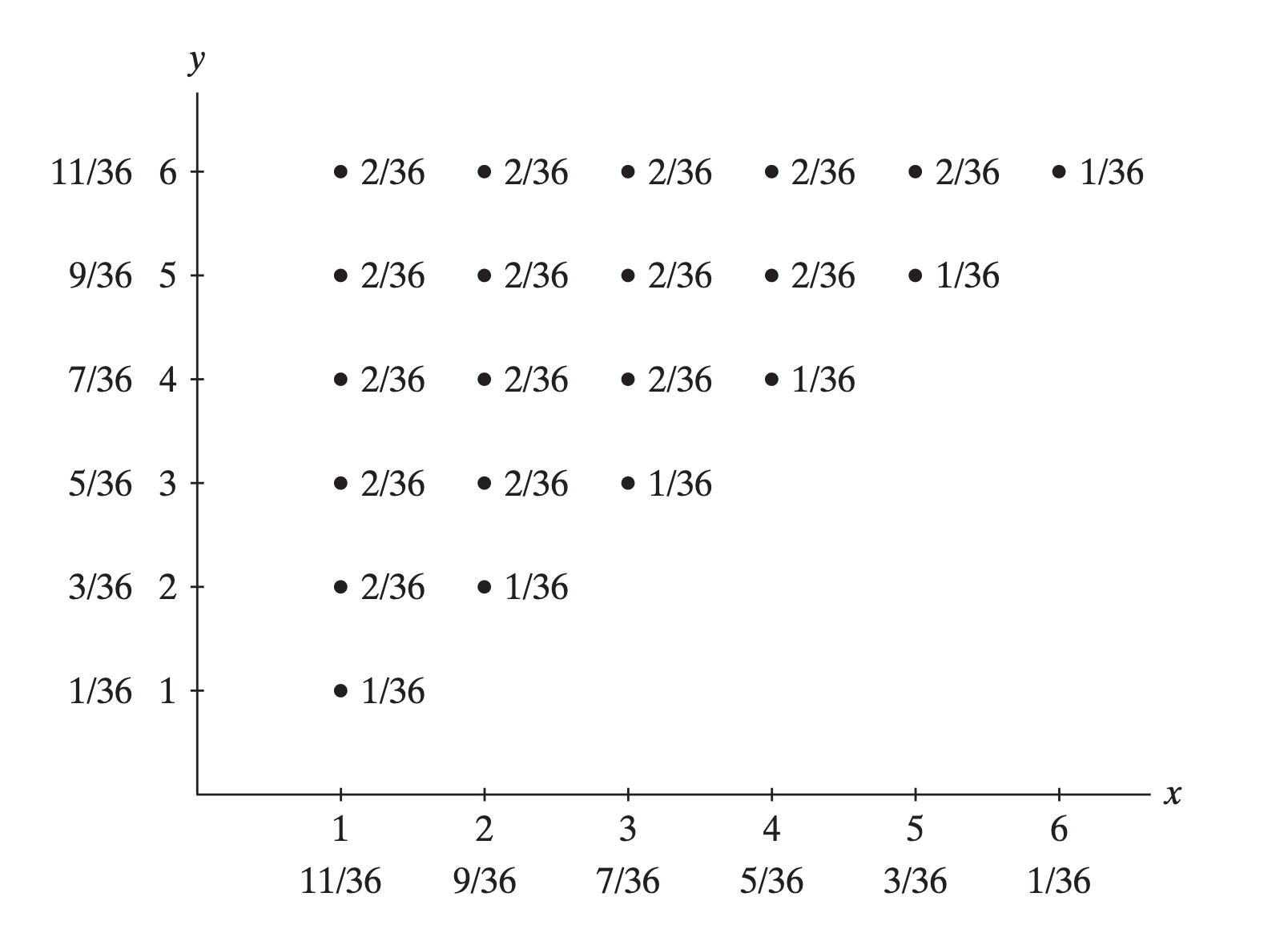
Figure 5.17: Joint p.m.f. for \(X\) and \(Y\) in the dice example [11].
Compute \(P(X=a)\) and \(P(Y=b)\), for \(a,b=1,\ldots, 6\).
Answer: for every \(a=1,\ldots,6\), \(\{X=a\}\) corresponds to the following union of events: \[\begin{aligned} \{X=a,Y=a\}\cup &\{X=a,Y=a+1\}\cup \cdots \\ &\cdots \cup \{X=a,Y=6\}.\end{aligned}\] These events are mutually exclusive, so that \[\begin{aligned} P(X=a)&=\sum_{y=a}^6P(\{X=a,Y=y\})\\&=\frac{1}{36}+\sum_{y=a+1}^6\frac{2}{36} \\ &=\frac{1}{36}+\frac{2(6-a)}{36}, \quad a=1,\ldots, 6.\end{aligned}\] Similarly, we get \[P(Y=b)=\frac{1}{36}+\frac{2(b-6)}{36},\ b=1,\ldots, 6.\] These marginal probabilities can be found in the margins of the p.m.f.
Compute \(P(X=3\mid Y>3)\), \(P(Y\le 3 \mid X\geq 4)\).
Answer: the notation suggests how to compute these conditional probabilities: \[\begin{aligned} P(X=3\mid Y>3)&=\frac{P(X=3 \cap Y>3)}{P(Y>3)} \\ P(Y=3|X\geq 4)&=\frac{P(Y=3 \cap X\geq 4)}{P(X \geq 4)}\end{aligned}\] The region corresponding to \(P(Y>3)=\frac{27}{36}\) is shaded in red (see image at the top of the following column); the region corresponding to \(P(X=3)=\frac{7}{36}\) is shaded in blue. The region corresponding to \[P(X=3\cap Y>3)=\frac{6}{36}\] is the intersection of the regions: \[P(X=3\mid Y>3)=\frac{6/36}{27/36}=\frac{6}{27}\approx 0.2222.\] As \(P(Y\le 3\cap X\ge 4)=0\), \(P(Y\le 3|X\ge 4)=0\).
Figure 5.18: Conditional probabilities in the dice example [11].
Are \(X\) and \(Y\) independent?
Answer: why didn’t we simply use the multiplicative rule to compute \[P(X=3 \cap Y>3)=P(X=3)P(Y>3)?\] It’s because \(X\) and \(Y\) are not independent, that is, it is not always the case that \[P(X=x,Y=y)=P(X=x)P(Y=y)\] for all allowable \(x,y\).
As it is, \(P(X=1,Y=1)=\frac{1}{36}\), but \[P(X=1)P(Y=1)=\frac{11}{36}\cdot \frac{1}{36}\neq \frac{1}{36},\] so \(X\) and \(Y\) are dependent (this is often the case when the domain of the joint p.d.f./p.m.f. is not rectangular).
There are \(8\) similar chips in a bowl: three marked \((0,0)\), two marked \((1,0)\), two marked \((0,1)\) and one marked \((1,1)\). A player selects a chip at random and is given the sum of the two coordinates, in dollars (taken from [11]).
What is the joint probability mass function of \(X_1\), and \(X_2\)?
Answer: let \(X_1\) and \(X_2\) represent the coordinates; we have \[f(x_1,x_2)=\frac{3-x_1-x_2}{8},\quad x_1,x_2=0,1.\]
What is the expected pay-off for this game?
Answer: the pay-off is simply \(X_1+X_2\). The expected pay-off is thus \[\begin{aligned} \text{E}[X_1+X_2]&=\sum_{x_1=0}^1\sum_{x_2=1}^0(x_1+x_2)f(x_1,x_2)\\&=0\cdot \frac{3}{8}+1\cdot\frac{2}{8}+1\cdot \frac{2}{8}+2\cdot \frac{1}{8}\\&=0.75. \end{aligned}\]
Let \(X\) and \(Y\) have joint p.d.f. \[f(x,y)=2,\quad 0\leq y\leq x\leq 1.\]
What is the support of \(f(x,y)\)?
Answer: the support is the set \(S=\{(x,y):0\leq y\leq x\leq 1\}\), a triangle in the \(xy\) plane bounded by the \(x-\)axis, the line \(y=1\), and the line \(y=x\).
The support is the blue triangle shown below.
Figure 5.19: Support for the joint distribution of \(X\) and \(Y\) in the above example.
What is \(P(0\leq X\leq 0.5, 0\leq Y\leq 0.5)\)?
Answer: we need to evaluate the integral over the shaded area: \[\begin{aligned} P(0\leq &X\leq 0.5,0\leq Y\leq 0.5)\\&=P(0\leq X\leq 0.5,0\leq Y\leq X)\\& =\int_{0}^{0.5}\int_{0}^x2\, dydx\\&=\int_0^{0.5}\left[2y\right]_{y=0}^{y=x}\, dx \\ & =\int_{0}^{0.5}2x\, dx=1/4.\end{aligned}\]
What are the marginal probabilities \(P(X=x)\) and \(P(Y=y)\)?
Answer: for \(0\leq x\leq 1\), we get \[\begin{aligned} P(X=x)&=\int_{-\infty}^{\infty}f(x,y)\, dy\\ &=\int_{y=0}^{y=x}2\, dy=\left[2y\right]_{y=0}^{y=x}=2x, \end{aligned}\] and for \(0\leq y\leq 1\), \[\begin{aligned} P(Y=y)&=\int_{-\infty}^{\infty}f(x,y)\, dx=\int_{x=y}^{x=1}2\, dx\\ &=\left[2x\right]_{x=y}^{x=1}=2-2y.\end{aligned}\]
Compute \(\text{E}[X]\), \(\text{E}[Y]\), \(\text{E}[X^2]\), \(\text{E}[Y^2]\), and \(\text{E}[XY]\).
Answer: we have \[\begin{aligned} \text{E}[X]&=\iint_Sxf(x,y)\, dA =\int_{0}^{1}\int_{0}^x2x\, dydx\\&=\int_0^1\left[2xy\right]_{y=0}^{y=x}\, dx = \int_{0}^1 2x^2\, dx \\&=\left[\frac{2}{3}x^3\right]_{0}^{1}=\frac{2}{3};\\ \text{E}[Y]&=\iint_Syf(x,y)\, dA =\int_{0}^{1}\int_{y}^12y\, dxdy\\&=\int_0^1\left[2xy\right]_{x=y}^{x=1}\, dy = \int_{0}^1 (2y-2y^2)\, dy \\&=\left[y^2-\frac{2}{3}y^3\right]_{0}^{1}=\frac{1}{3}; \\ \text{E}[X^2]&=\iint_Sx^2f(x,y)\, dA =\int_{0}^{1}\int_{0}^x2x^2\, dydx\\&=\int_0^1\left[2x^2y\right]_{y=0}^{y=x}\, dx = \int_{0}^1 2x^3\, dx \\&=\left[\frac{1}{2}x^4\right]_{0}^{1}=\frac{1}{2};\\ \text{E}[Y^2] &= \iint_Sy^2f(x,y)\, dA =\int_{0}^{1}\int_{y}^12y^2\, dxdy\\&=\int_0^1\left[2xy^2\right]_{x=y}^{x=1}\, dy = \int_{0}^1 (2y-2y^3)\, dy \\&=\left[\frac{2}{3}y^3-\frac{1}{2}y^4\right]_{0}^{1}=\frac{1}{6};\\ \text{E}[XY]&=\iint_Sxyf(x,y)=\int_{0}^1\int_{0}^x2xy\, dydx\\&=\int_0^2\left[xy^2\right]_{y=0}^{y=x}=\int_{0}^1x^2\, dx \\ &=\left[\frac{x^4}{4}\right]_{0}^1=\frac{1}{4}.\end{aligned}\]
Are \(X\) and \(Y\) independent?
Answer: they are not independent as the support of the joint p.d.f. is not rectangular.
The covariance of two random variables \(X\) and \(Y\) can give some indication of how they depend on one another: \[\begin{aligned} \text{Cov}(X,Y)&=\text{E}[(X-\text{E}[X])(Y-\text{E}[Y])]\\&=\text{E}[XY]-\text{E}[X]\text{E}[Y].\end{aligned}\] When \(X=Y\), the covariance reduces to the variance.15
Example: in the last example, \(\text{Var}[X]=\frac{1}{2}-(\frac{2}{3})^2=\frac{1}{18}\), \(\text{Var}[X]=\frac{1}{6}-(\frac{1}{3})^2=\frac{1}{18}\), and \(\text{Cov}(X,Y)=\frac{1}{4}-\frac{2}{3}\cdot\frac{1}{3}=\frac{1}{36}\).
In R, we can generate a multivariate joint normal via MASS’s mvrnorm(), whose required paramters are n, a mean vector mu and a covariance matrix Sigma.
We’ll sample 1000 observations from the joint normal \(N(\mu,\Sigma)\).
'data.frame':   1000 obs. of  2 variables:
 $ X1: num  -1.038 -2.427 -1.181 -0.221 -0.966 ...
 $ X2: num  0.325 1.526 0.13 0.3 0.274 ...
# let's plot the data... what would you expect to see here?
library(ggplot2)
library(hexbin)
qplot(X1, X2, data=a, geom="hex")
The covariance matrix was diagonal, so we expect theblob to be circular. What happens if we use a non-diagonalcovariance matrix?
mu = c(-3,12)
Sigma = matrix(c(110,15,15,3),2,2)
a<-mvrnorm(1000,mu,Sigma)
a<-data.frame(a)
qplot(X1, X2, data=a, geom="hex") + ylim(-40,40) + xlim(-40,40)
5.5 Central Limit Theorem and Sampling Distributions
In this section, we introduce one of the fundamental results of probability theory and statistical analysis.
5.5.1 Sampling Distributions
A population is a set of similar items which of interest in relation to some questions or experiments.
In some situations, it is impossible to observe the entire set of observations that make up a population – perhaps the entire population is too large to query, or some units are out-of-reach.
In these cases, we can only hope to infer the behaviour of the entire population by considering a sample (subset) of the population.
Suppose that \(X_1,\ldots,X_n\) are \(n\) independent random variables, each having the same c.d.f.\(F\), i.e.they are identically distributed. Then, \(\{X_1,\ldots,X_n\}\) is a random sample of size \(n\) from the population, with c.d.f.\(F\,.\)
Any function of such a random sample is called a statistic of the sample; the probability distribution of a statistic is called a sampling distribution.
Recall the linear properties of the expectation and the variance: if \(X\) is a random variable and \(a,b\in \mathbb{R}\), then \[\begin{aligned} \text{E}\left[ a+bX \right]&= a+b\text{E}[X]\,,\\ \text{Var}\left[ a+bX \right]&= b^2\text{Var}[X]\,,\\ \text{SD}\left[ a+bX \right]&=|b|\text{SD}[X]\,.\end{aligned}\]
Sum of Independent Random Variables
For any random variables \(X\) and \(Y\), we have \[\text{E}[X+Y]= \text{E}[X]+\text{E}[Y].\] In general, \[\text{Var}[X+Y]=\text{Var}[X]+2\text{Cov}(X,Y)+\text{Var}[Y];\] if in addition \(X\) and \(Y\) are independent, then \[\text{Var}[X+Y]=\text{Var}[X]+\text{Var}[Y].\] More generally, if \(X_1,X_2,\ldots,X_n\) are independent, then \[\text{E}\left[ \sum_{i=1}^nX_i \right]=\sum_{i=1}^n \text{E}[X_i] \quad\text{and}\quad \text{Var}\left[ \sum_{i=1}^nX_i \right]=\sum_{i=1}^n \text{Var}[X_i]\,.\]
Independent and Identically Distributed Random Variables
A special case of the above occurs when all of \(X_1,\ldots,X_n\) have exactly the same distribution. In that case we say they are independent and identically distributed, which is traditionally abbreviated to “iid”. If \(X_1,\ldots,X_n\) are iid, and \[\begin{aligned} \text{E}\left[ X_i \right] = \mu&\quad\text{and}&\text{Var}\left[ X_i \right]=\sigma^2 \quad\text{for }i=1,\ldots,n,\end{aligned}\] then \[\begin{aligned} \text{E}\left[ \sum_{i=1}^nX_i \right]=n\mu&\quad\text{and}& \text{Var}\left[ \sum_{i=1}^n X_i \right]=n\sigma^2\,.\end{aligned}\]
Examples
A random sample of size \(100\) is taken from a population with mean \(50\) and variance \(0.25\). Find the expected value and variance of the sample total.
Answer: this problem translates to "if \(X_1,\ldots,X_{100}\) are iid with \(\text{E}[X_i]=\mu=50\) and \(\text{Var}[X]=\sigma^2=0.25\) for \(i=1,\ldots,100\), find \(\text{E}\left[\tau\right]\) and \(\text{Var}\left[\tau \right]\) for \[\tau=\sum_{i=1}^nX_i.\text{''}\] According to the iid formulas, \[\begin{aligned} \text{E}\left[\sum_{i=1}^nX_i \right]&= 100\mu=5000 \\ \text{Var}\left[\sum_{i=1}^nX_i \right] &= 100\sigma^2=25\,.\end{aligned}\]
The mean value of potting mix bags weights is \(5\) kg, with standard deviation \(0.2\). If a shop assistant carries \(4\) bags (selected independently from stock) then what is the expected value and standard deviation of the total weight carried?
Answer: there is an implicit “population” of bag weights. Let \(X_1,X_2,X_3,X_4\) be iid with \(\text{E}[X_i]=\mu=5\), \(\text{SD}[X_i]=\sigma=0.2\) and \(\text{Var}[X_i]=\sigma^2=0.2^2 = 0.04\) for \(i=1,2,3,4\). Let \(\tau=X_1+X_2+X_3+X_4\).
According to the iid formulas, \[\begin{aligned} \text{E}[\tau]&= n\mu=4\cdot 5=20 \\ \text{Var}[\tau]&=n\sigma^2=4\cdot0.04=0.16.\end{aligned}\] Thus, \(\text{SD}[\tau]=\sqrt{0.16}=0.4\).
Sample Mean
The sample mean is a typical statistic of interest: \[\overline{X} = \frac1n\sum_{i=1}^nX_i\,.\] If \(X_1, \ldots, X_n\) are iid with \(\text{E}[X_i]=\mu\) and \(\text{Var}[X_i]=\sigma^2\) for all \(i=1,\ldots, n\), then $$ \[\begin{aligned} \text{E}\left[ \overline{X} \right]&= \text{E}\left[ \frac1n \sum_{i=1}^nX_i \right]=\frac1n\text{E}\left[\sum_{i=1}^nX_i \right]=\frac1n\left( n\mu \right)=\mu\, \\ \text{Var}\left[ \overline{X} \right]&= \text{Var}\left[ \frac1n \sum_{i=1}^nX_i \right]= \frac{1}{n^2}\text{Var}\left[\sum_{i=1}^nX_i \right]=\frac{1}{n^2}\left( n\sigma^2 \right)=\frac{\sigma^2}n\,.\end{aligned}\]$$
Example: a set of scales returns the true weight of the object being weighed plus a random error with mean \(0\) and standard deviation \(0.1\) g. Find the standard deviation of the average of \(9\) such measurements of an object.
Answer: suppose the object has true weight \(\mu\). The “random error” indicates that each measurement \(i=1,\ldots, 9\) is written as \(X_i=\mu+Z_i\) where \(\text{E}[Z_i]=0\) and \(\text{SD}[Z_i]=0.1\) and the \(Z_i\)’s are iid.
The \(X_i\)’s are iid with \(\text{E}[X_i]=\mu\) and \(\text{SD}[X_i]=\sigma=0.1\). If we average \(X_1,\ldots,X_n\) (with \(n=9\)) to get \(\overline{X}\), then \[\begin{aligned} \text{E}\left[ \overline{X} \right] = \mu~~~\text{and}~~~ \textstyle \text{SD}\left[ \overline{X} \right]=\frac{\sigma}{\sqrt n} = \frac{0.1}{\sqrt{9}}=\frac1{30}\approx0.033\,.\end{aligned}\] We do not need to know the actual distribution of the \(X_i\); only \(\mu\) and \(\sigma^2\) are required to compute \(\text{E}[\overline{X}]\) and \(\text{Var}[\overline{X}]\).
Sum of Independent Normal Random Variables
Another interesting case occurs when we have multiple independent normal random variables on the same experiment.
Suppose \(X_i\sim\mathcal{N}\left(\mu_i,\sigma_i^2\right)\) for \(i=1,\ldots,n\), and all the \(X_i\) are independent. We already know that \[\begin{aligned} \text{E}[\tau]&= \text{E}[X_1+\cdots+X_n]=\text{E}[X_1]+\cdots+\text{E}[X_n]=\mu_1+\cdots+\mu_n\,; \\ \text{Var}[\tau]&=\text{Var}[X_1+\cdots+X_n]=\text{Var}[X_1]+\cdots+\text{Var}[X_n]=\sigma^2_1+\cdots+\sigma^2_n\,.\end{aligned}\] It turns out that, under these hypotheses, \(\tau\) is also normally distributed, i.e. \[{\tau=\sum_{i=1}^nX_i \sim\mathcal{N}(\text{E}[\tau],\text{Var}[\tau])=\mathcal{N}\left( \mu_1+\cdots+\mu_n,\sigma_1^2+\cdots+\sigma_n^2 \right)}.\] Thus, if \(\{X_1,\ldots,X_n\}\) is a random sample from a normal population with mean \(\mu\) and variance \(\sigma^2\), then \(\sum_{i=1}^nX_i\) and \(\overline{X}\) are also normal, which, combined with the above work, means that \[\begin{aligned} \sum_{i=1}^nX_i\sim\mathcal{N}\left( n\mu,n\sigma^2 \right)&\quad\text{and}& \overline{X}\sim\mathcal{N}\left( \mu,\frac{\sigma^2}n \right)\,.\end{aligned}\]
Example: suppose that the population of students’ weights is normal with mean \(75\) kg and standard deviation \(5\) kg. If \(16\) students are picked at random, what is the distribution of the (random) total weight \(\tau\)? What is the probability that the total weight exceeds \(1250\) kg?
Answer: If \(X_1,\ldots,X_{16}\) are iid as \(\mathcal{N}(75,25)\), then the sum \(\tau=X_1+\cdots + X_{16}\) is also normally distributed with \[\tau=\sum_{i=1}^{16}X_i\sim\mathcal{N}(16\cdot 75,16\cdot 25)=\mathcal{N}(1200,400),\quad\text{and}\] \[Z=\frac{\tau -1200}{\sqrt{400}}\sim\mathcal{N}(0,1).\] Thus, \[SD1\] \[\begin{aligned} P(\tau >1250) &= P\left( \frac{\tau -1200}{\sqrt{400}}>\frac{1250-1200}{20} \right)\\&=P(Z>2.5)=1-P(Z\leq2.5)\\&\approx1-0.9938=0.0062\,.\end{aligned}\]
5.5.2 Central Limit Theorem
Suppose that a professor has been teaching a course for the last 20 years. For every cohort during that period, the mid-term exam grades of all the students have been recorded. Let \(X_{i,j}\) be the grade of student \(i\) in year \(j\). Looking back on the class lists, they find that \[\text{E}[X_{i,j}]=56\quad\mbox{and} \quad \text{SD}[X_{i,j}]=11.\] This year, there are \(49\) students in the class. What should the professor expect for the class mid-term exam average?
Of course, the professor cannot predict any of the student grades or the class average with absolute certainty, but they could try the following approach:
simulate the results of the class of \(49\) students by generating sample grades \(X_{1,1},\ldots, X_{1,49}\) from a normal distribution \(\mathcal{N}(65,15^2)\);
compute the sample mean for the sample and record it as \(\overline{X}_1\);
repeat steps 1-2 \(m\) times and compute the standard deviation of the sample means \(\overline{X}_1,\ldots,\overline{X}_m\);
plot the histogram of the sample means \(\overline{X}_1,\ldots,\overline{X}_m\).
What do you think is going to happen?
Central Limit Theorem: If \(\overline{X}\) is the mean of a random sample of size \(n\) taken from an unknown population with mean \(\mu\) and finite variance \(\sigma^2\,,\) then \[Z=\frac{\overline{X}-\mu}{\sigma/\sqrt{n}}\sim \mathcal{N}(0,1),\] as \(n\to\infty\).
More precisely, this is a limiting result. If we view the standardization \[Z_n =\frac{\overline{X} - \mu}{\sigma/\sqrt n},\] as functions of \(n\), we have, for each \(z\), \[\begin{aligned} \lim_{n\to\infty}P\left( Z_n\leq z \right)&=\Phi(z)~~~\text{and}\\ P\left( Z_n\leq z \right)&\approx \Phi(z), \text{ if $n$ is large enough},\end{aligned}\] whether the original \(X_i\)’s are normal or not.

Figure 5.20: Illustration of the central limit theorem with a normal underlying distribution and with an exponential underlying distribution [source unknown].
Examples
The examination scores in an university course have mean \(56\) and standard deviation \(11\). In a class of \(49\) students, what is the probability that the average mark is below \(50\)? What is the probability that the average mark lies between \(50\) and \(60\)?
Answer: let the marks be \(X_1,..., X_{49}\) and assume the performances are independent. According to the central limit theorem, \[\overline{X} = (X_1 + X_2 + \cdots + X_{49})/49,\] with \(\text{E}[\overline{X}]=56\) and \(\text{Var}[\overline{X}]= 11^2 /49\). We thus have \[\begin{aligned} P(\overline{X} < 50) &\approx P\left(Z < \frac{50 -56}{11/7}\right)\\&= P(Z < -3.82) = 0.0001\end{aligned}\] and \[\begin{aligned} P(50 < \overline{X} < 60) &\approx P\left( \frac{50 -56}{11/7} < Z < \frac{60-56}{11/7}\right)\\ &= P( -3.82 < Z < 2.55)\\&=\Phi(2.55) - \Phi(-3.82)\\&= 0.9945.\end{aligned}\] Note that this says nothing about whether the scores are normally distributed or not, only that the average scores follow an approximate normal distribution.16
Systolic blood pressure readings for pre-menopausal, non-pregnant women aged \(35 - 40\) have mean \(122.6\) standard deviation \(11\) mm Hg. An independent sample of \(25\) women is drawn from this target population and their blood pressure is recorded.
What is the probability that the average blood pressure is greater than \(125\) mm Hg? How would the answer change if the sample size increases to \(40\)?
Answer: according to the CLT, \(\overline{X} \sim \mathcal{N}( 122.6, 121/25)\), approximately. Thus \[\begin{aligned} P(\overline{X} > 125) & \approx P\left(Z > \frac{125-122.6}{11/\sqrt{25}}\right)\\ & = P(Z > 1.09) = 1-\Phi(1.09)\\&=0.14.\end{aligned}\] However, if the sample size is \(40\), then \[\begin{aligned} P(\overline{X} > 125) & \approx P\left(Z > \frac{125-122.6}{11/\sqrt{40}}\right)=0.08.\end{aligned}\] Increasing the sample size reduces the probability that the average is far from the expectation of each original measurement.
Suppose that we select a random sample \(X_1,\ldots,X_{100}\) from a population with mean \(5\) and variance \(0.01\).
What is the probability that the difference between the sample mean of the random sample and the mean of the population exceeds \(0.027\)?
Answer: according to the CLT, we know that, approximately, \(Z=\frac{\overline{X}-\mu}{\sigma/\sqrt{n}}\) has standard normal distribution. The desired probability is thus \[\begin{aligned} P&=P(|\overline{X}-\mu|\ge 0.027)\\&=P(\overline{X}-\mu\ge 0.027 \text{ or }\mu-\overline{X}\ge 0.027)\\&=P\left(\frac{\overline{X}-5}{0.1/\sqrt{100}}\ge \frac{0.027}{0.1/\sqrt{100}}\right)\\ & \ \ \ \ \ \ \ \ \ \ \ \ \ \ \ \ \ \ \ +P\left(\frac{\overline{X}-5}{0.1/\sqrt{100}}\le \frac{-0.027}{0.1/\sqrt{100}}\right)\\ &\approx P\left(Z\ge 2.7\right)+P\left(Z\le -2.7\right)\\&=2P\left(Z\ge 2.7\right)\approx 2(0.0035)=0.007.\end{aligned}\]
In the next example, we illustrate how to use the Central Limit Theorem with R.
Example: a large freight elevator can transport a maximum of 9800 lbs. Suppose a load containing 49 boxes must be transported. From experience, the weight of boxes follows a distribution with mean \(\mu=205\) lbs and standard deviation \(\sigma=15\) lbs. Estimate the probability that all 49 boxes can be safely loaded onto the freight elevator and transported.
Solution: we are given \(n=49\), \(\mu=205\), and \(\sigma=15\). Let us further assume that the boxes all come from different sources (i.e. the boxes’ weight \(x_i\), \(i=1,\ldots,49\), are independent of one another)
To get a sense of the task’s feasibility, we simulate a few scenarios. Note that the problem makes no mention of the type of distribution that the weights follow.
To start, we assume that the weights are normally distributed.
set.seed(0) # to ensure replicability
x<-rnorm(49,mean=205,sd=15)

brks = seq(min(x),max(x),(max(x)-min(x))/10)
hist(x, breaks = brks)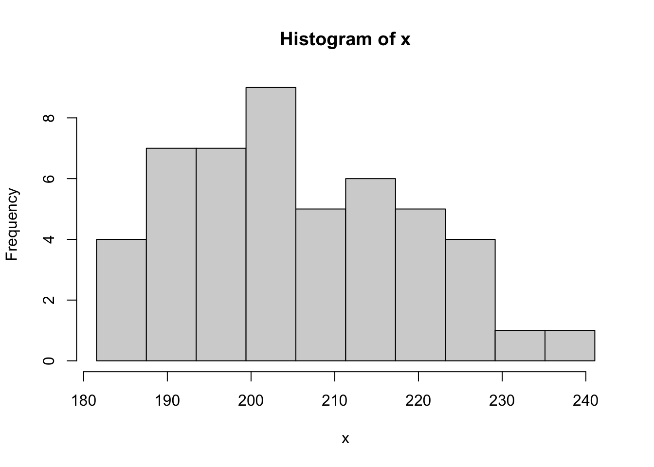
The elevator can transport up to 9800 lbs; the \(n=49\) boxes can be transported if their total weight \[T=49w=x_1+\cdots +x_{49},\] where \(w=\overline{x}\), is less than 9800 lbs. In mathematical terms, we are interested in the value of the probability \(P(T<9800)\).
For the sample x from above, we get:
[1] 10066.36and so that specific group of 49 boxes would be too heavy to carry in one trip.
Perhaps we were simply unlucky – perhaps another group of boxes would have been light enough. Let us try again, but with a different group of boxes.
[1] 9852.269It’s close, but no cigar. However, two tries are not enough to establish a trend and to estimate \(P(T<9800)\).
Wewrite a little function to help us find an estimate of the probability. The idea is simple: if we were to try a large number of random combinations of 49 boxes, the proportion of the attempts for which the total weight \(T\) falls below 9800 is (hopefully?) going to approximate \(P(T<9800)\).
# see if you can figure out what kind of inputs these are meant to be, and what this code does
# running this cell will compile the function, but
# it still needs to be called with appropriate inputs to provide an estimate for P(T<9800)

estimate_T.normal <- function(n, T.threshold, mean, sd, num.tries){
  a=0
  for(j in 1:num.tries){
    if(sum(rnorm(n,mean=mean,sd=sd))<T.threshold){
      a=a+1
    }
  }
  estimate_T.normal <- a/num.tries
}
We try the experiment 10, 100, 1000, 10000, 100000, and 1000000 times.
(c(estimate_T.normal(49,9800,205,15,10),
estimate_T.normal(49,9800,205,15,100),
estimate_T.normal(49,9800,205,15,1000),
estimate_T.normal(49,9800,205,15,10000),
estimate_T.normal(49,9800,205,15,100000),
estimate_T.normal(49,9800,205,15,1000000)))
[1] 0.00000 0.01000 0.00700 0.00990 0.00973 0.00975We cannot say too much from such a simple set up, but it certainly seems as though we should expect success about \(1\%\) of the time.
That is a low probability, which suggests that 49 is too many boxes for the elevator to work correctly, in general, but perhaps that is only the case because we assumed normality. What happens if we used other distributions with the same characteristics, such as \(U(179.0192379,230.9807621)\) or \(\Lambda(5.320340142,0.005339673624)\)?
(How would we verify that these distributions indeed have the right characteristics? How would we determine the appropriate parameters in the first place?)
Let us try with those two distributions.
estimate_T.unif <- function(n, T.threshold, min, max, num.tries){
  a=0
  for(j in 1:num.tries){
    if(sum(runif(n,min=min,max=max))<T.threshold){
      a=a+1
    }
  }
estimate_T.unif <- a/num.tries
}

(c(estimate_T.unif(49,9800,179.0192379,230.9807621,10),
 estimate_T.unif(49,9800,179.0192379,230.9807621,100),
 estimate_T.unif(49,9800,179.0192379,230.9807621,1000),
 estimate_T.unif(49,9800,179.0192379,230.9807621,10000),
 estimate_T.unif(49,9800,179.0192379,230.9807621,100000),
 estimate_T.unif(49,9800,179.0192379,230.9807621,1000000)))
[1] 0.000000 0.010000 0.008000 0.007900 0.010230 0.009613estimate_T.lnorm <- function(n, T.threshold, meanlog, sdlog, num.tries){
a=0
for(j in 1:num.tries){
if(sum(rlnorm(n,meanlog=meanlog,sdlog=sdlog))<T.threshold){
a=a+1
}
}
estimate_T.lnorm <- a/num.tries
}
(c(estimate_T.lnorm(49,9800,5.320340142,sqrt(0.005339673624),10),
estimate_T.lnorm(49,9800,5.320340142,sqrt(0.005339673624),100),
estimate_T.lnorm(49,9800,5.320340142,sqrt(0.005339673624),1000),
estimate_T.lnorm(49,9800,5.320340142,sqrt(0.005339673624),10000),
estimate_T.lnorm(49,9800,5.320340142,sqrt(0.005339673624),100000),
estimate_T.lnorm(49,9800,5.320340142,sqrt(0.005339673624),1000000)))[1] 0.000000 0.000000 0.006000 0.009500 0.009060 0.009184Under all three distributions, it appears as though \(P(T<9800)\) converges to a value near \(1\%\), even though the three distributions are very different. That might be surprising at first glance, but it is really a consequence of the Central Limit Theorem.
In effect, we are interested in estimating \(P(T<9800)=P(w<9800/49)=P(w<200)\), where \(w\) is the mean weight of the boxes.
According to the CLT, the distribution of \(w\) is approximately normal with mean \(\mu=205\) and variance \(\sigma^2/n=15^2/49\), even if the weights themselves were not normally distributed.
By subtracting the mean of \(w\) and dividing by the standard deviation we obtain a new random variable \(z\) which is approximately the standard unit normal, i.e. \[P(w<200)\approx P\left(z<\frac{200−205}{15/7}\right).\]
[1] -2.333333Thus, \(P(w<200)\approx P(z<−2.33)\) and we need to find the probability that the standard normal p.d.f. is smaller than \(-2.33\).
This can be calculated with the pnorm() function:
[1] 0.009903076Hence, \(P(T<9800)\approx 0.0099\), which means that it is highly unlikely that the 49 boxes can be transported in the elevator all at once.
Example: what elevator threshold would be required to reach a probability of success of \(10\%\)? \(50\%\)? \(75\%\)?
Answer: the following routine approximates the probability in question without resorting to simulating the weights (that is, independently of the underlying distribution of weights) for given n, threshold, mean, and sd. Can you figure out what pnorm() is doing?
prob_T <- function(n,threshold,mean,sd){
  prob_T=pnorm((threshold/n - mean)/(sd/sqrt(n)),0,1)
}

max(which(prob_T(49,1:12000,205,15)<0.1))
max(which(prob_T(49,1:12000,205,15)<0.5))
max(which(prob_T(49,1:12000,205,15)<0.75))

plot((prob_T(49,1:12000,205,15)))
[1] 9910
[1] 10044
[1] 10115
5.5.3 Sampling Distributions (Reprise)
We now revisit sampling distributions.
Difference Between Two Means
Statisticians are often interested in the difference between various populations; a result akin to the central limit theorem provides guidance in that area.
Theorem: Let \(\{X_1,\ldots,X_n\)} be a random sample from a population with mean \(\mu_1\) and variance \(\sigma_1^2\), and \(\{Y_1,\ldots,Y_m\}\) be another random sample, independent of \(X\), from a population with mean \(\mu_2\) and variance \(\sigma_2^2\).
If \(\overline{X}\) and \(\overline{Y}\) are the respective sample means, then \[Z=\frac{\overline{X}-\overline{Y}-(\mu_1-\mu_2)}{\sqrt{\frac{\sigma_1^2}{n}+\frac{\sigma_2^2}{m}}}\] has standard normal distribution \(\mathcal{N}(0,1)\) as \(n,m\to\infty\).17
Example: two different machines are used to fill cereal boxes on an assembly line. The critical measurement influenced by these machines is the weight of the product in the boxes.
The variances of these weights is identical, \(\sigma^2=1\). Each machine produces a sample of \(36\) boxes, and the weights are recorded. What is the probability that the difference between the respective averages is less than \(0.2\), assuming that the true means are identical?
we have \(\mu_1=\mu_2\), \(\sigma_1^2=\sigma_2^2=1\), and \(n=m=36\). The desired probability is \[\begin{aligned} P&\left(|\overline{X}-\overline{Y}|<0.2\right)=P\left(-0.2<\overline{X}-\overline{Y}<0.2\right)\\&=P\left(\frac{-0.2-0}{\sqrt{1/36+1/36}}<\frac{\overline{X}-\overline{Y}-(\mu_1-\mu_2)}{\sqrt{1/36+1/36}}<\frac{0.2-0}{\sqrt{1/36+1/36}}\right)\\ &=P(-0.8485<Z<0.8485)\\&\approx\Phi(0.8485)-\Phi(-0.8485)\approx 0.6.\end{aligned}\]
Sample Variance \(S^2\)
When the underlying variance is unknown (which is usually the case in practice), it must be approximated by the sample variance.
Theorem: Let \(\{X_1,\ldots,X_n\}\) be a random sample taken from a normal population with mean \(\sigma^2\), and \[S^2=\frac{1}{n-1}\sum_{i=1}^n (X_i-\overline{X})^2\] be the sample variance. The statistic \[\chi^2=\frac{(n-1)S^2}{\sigma^2}=\sum_{i=1}^n\frac{(X_i-\overline{X})^2}{\sigma^2}\] follows a chi-squared distribution with \(\nu=n-1\) degrees of freedom (d.f.), where \(\chi^2(\nu)=\Gamma(1/2,\nu)\).
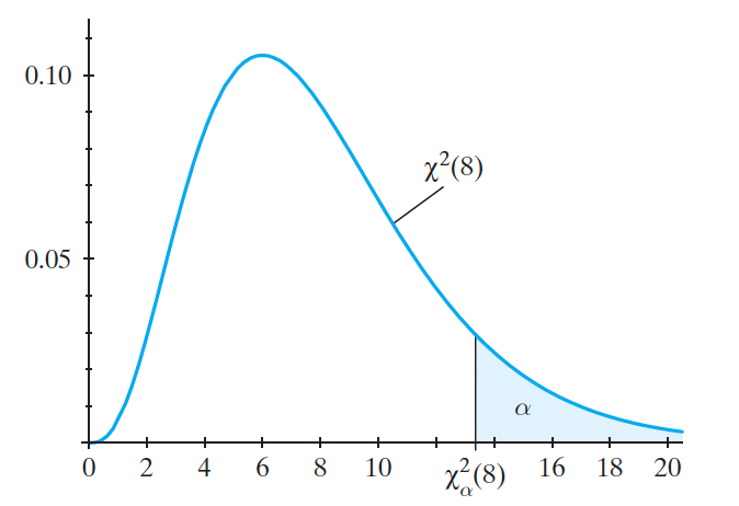
Figure 5.21: Chi-squared distribution with 8 degrees of freedom [11].
Notation: for \(0<\alpha<1\) and \(\nu \in \mathbb{N}^*\), \(\chi^2_\alpha(\nu)\) is the critical value for which \[P(\chi^2>\chi^2_\alpha(\nu))=\alpha\,,\] where \(\chi^2\sim \chi^2(\nu)\) follows a chi-squared distribution with \(\nu\) degrees of freedom.
The values of \(\chi^2_\alpha(\nu)\) can be found in various textbook
tables, or by using R or specialized online calculators.
For instance, when \(\nu=8\) and \(\alpha=0.95\), we compute \(\chi^2_{0.95}(8)\) via
[1] 2.732637so that \(P(\chi^2>2.732)=0.95\,,\) where \(\chi^2\sim \chi^2(8)\), i.e., \(\chi^2\) has a chi-squared distribution with \(\nu=8\) degrees of freedom.
In other words, \(95\%\) of the area under the curve of the probability density function of \(\chi^2(8)\) is found to the right of \(2.732\).
Sample Mean With Unknown Population Variance
Suppose that \(Z\sim \mathcal{N}(0,1)\) and \(V\sim \chi^2(\nu)\). If \(Z\) and \(V\) are independent, then the distribution of the random variable \[T=\frac{Z}{\sqrt{V/\nu}}\] is a Student \(t-\)distribution with \(\nu\) degrees of freedom, which we denote by \(T\sim t(\nu)\).18
Theorem: let \(X_1,\ldots,X_n\) be independent normal random variables with mean \(\mu\) and standard deviation \(\sigma\,.\) Let \(\overline{X}\) and \(S^2\) be the sample mean and sample variance, respectively. Then the random variable \[T=\frac{\overline{X}-\mu}{S/\sqrt{n}}\sim t(n-1),\] follows a Student \(t-\)distribution with \(\nu=n-1\) degrees of freedom.
Using the same notation as with the chi-squared distribution, let \(t_\alpha(\nu)\) represent the critical \(t\)-value above which we find an area under the p.d.f. of \(t(\nu)\) equal to \(\alpha\,,\) i.e. \[P(T>t_\alpha(\nu))=\alpha\,,\] where \(T\sim t(\nu)\).
For all \(\nu\), the Student \(t\)-distribution is a symmetric distribution
around zero, so we have \(t_{1-\alpha}(\nu)=-t_\alpha(\nu).\) The critical
values can be found in tables, or by using the R function qt().
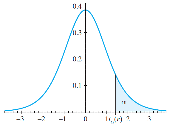
Figure 5.22: Student \(t-\)distribution with \(r\) degrees of freedom [11].
If \(T\sim t(\nu)\), then for any \(0<\alpha< 1\), we have \[\begin{aligned} P&\left(|T|<t_{\alpha/2}(\nu)\right)=P\left(-t_{\alpha/2}(\nu)<T<t_{\alpha/2}(\nu)\right)\\&=P\left(T<t_{\alpha/2}(\nu)\right)-P\left(T<-t_{\alpha/2}(\nu)\right)\\ &=1-P\left(T>t_{\alpha/2}(\nu)\right)-(1-P\left(T>-t_{\alpha/2}(\nu)\right))\\ &=1-P\left(T>t_{\alpha/2}(\nu)\right)-(1-P\left(T>t_{1-\alpha/2}(\nu)\right))\\ &=1-\alpha/2-(1-(1-\alpha/2))=1-\alpha.\end{aligned}\] Consequently, \[P\left(-t_{\alpha/2}(n-1)<\frac{\bar X-\mu}{S/\sqrt{n}}<t_{\alpha/2}(n-1)\right)=1-\alpha\,.\] We can show that \(t(\nu)\to \mathcal{N}(0,1)\) as \(\nu\to\infty\); intuitively, this makes sense because the estimate \(S\) gets better at estimating \(\sigma\) when \(n\) increases.
Example: in R, we can see that when \(T\sim t(8)\),
[1] 2.306004so that \(P\left( T>2.306 \right)=0.025,\) which implies \[P\left(T< -2.306 \right) = 0.025\,\], so \(t_{0.025}(8)=2.306\) and \[\begin{aligned} P\left( |T|\leq 2.306 \right)&= P\left( -2.306\leq T\leq 2.306 \right)\\ &= 1 - P\left( T<- 2.306 \right) - P\left( T>2.306 \right) \\& =1-2P\left( T<- 2.306 \right)= 0.95\,.\end{aligned}\] The Student \(t-\)distribution will be useful when the time comes to compute confidence intervals and to do hypothesis testing (see Basics of Statistical Analysis).
5.5.3.1 \(F-\)Distributions
Let \(U\sim \chi^2(\nu_1)\) and \(V\sim \chi^2(\nu_2)\). If \(U\) and \(V\) are independent, then the random variable \[F=\frac{U/\nu_1}{V/\nu_2}\] follows an \(F\)-distribution with \(\nu_1\) and \(\nu_2\) degrees of freedom, which we denote by \(F\sim F(\nu_1,\nu_2)\).
The probability density function of \(F(\nu_1,\nu_2)\) is \[f(x)=\frac{\Gamma(\nu_1/2+\nu_2/2)(\nu_1/\nu_2)^{\nu_1/2}x^{\nu_1/2-1}}{\Gamma(\nu_1/2)\Gamma(\nu_2/2)(1+x\nu_1/\nu_2)^{\nu_1/2+\nu_2/2}},\quad x\geq 0.\]
Theorem: If \(S_1^2\) and \(S_2^2\) are the sample variances of independent random samples of size \(n\) and \(m\), respectively, taken from normal populations with variances \(\sigma_1^2\) and \(\sigma_2^2\,,\) then \[F=\frac{S_1^2/\sigma_1^2}{S_2^2/\sigma_2^2}\sim F(n-1,m-1)\] follows an \(F\)-distribution with \(\nu_1=n-1\), \(\nu_2=m-1\) d.f.
Notation: for \(0<\alpha<1\) and \(\nu_1,\nu_2\in \mathbb{N}^*\),
\(f_\alpha(\nu_1,\nu_2)\) is the critical value for which
\(P(F>f_\alpha(\nu_1,\nu_2))=\alpha\) where \(F\sim F(\nu_1,\nu_2)\).
Critical values can be found in tables, or by using the R function
\(\texttt{qf()}\).
It can be shown that \[f_{1-\alpha}(\nu_1,\nu_2)=\frac{1}{f_{\alpha}(\nu_2,\nu_1)};\] for instance, since
[1] 0.2463077then
\[f_{0.95}(6,10)=\frac1{f_{0.05}(10,6)}=\frac{1}{4.06}=0.246\,.\]
These distributions play a role in linear regression and ANOVA models (see ANOVA).
References
[5] E. Ghashim and P. Boily, “A Soft Introduction to Bayesian Data Analysis,” Data Science Report Series, 2020.
[6] E. T. Jaynes, Probability theory: The logic of science. Cambridge Press, 2003.
[7] A. Kolmogorov, Foundations of the theory of probability. Chelsea Publishing Company, 1933.
[8] Mathematical Association, UK, “An Aeroplane’s Guide to A Level Maths.”
[9] Wikipedia, “List of probability distributions,” 2021,Available: https://en.wikipedia.org/wiki/List\_of\_probability\_distributions
[10] R. E. Walpole, R. H. Myers, S. L. Myers, and K. Ye, Probability & statistics for engineers and scientists, 8th ed. Upper Saddle River: Pearson Education, 2007.
[11] R. V. Hogg and E. A. Tanis, Probability and statistical inference, 7th ed. Pearson/Prentice Hall, 2006.
Events can be represented graphically using Venn diagrams – mutually exclusive events are those which do not have a common intersection.↩︎
This is a purely mathematical definition, but it agrees with the intuitive notion of independence in simple examples.↩︎
Is it clear what is meant by ``independent tosses’’?↩︎
What are some realistic values of \(p\)?↩︎
There is nothing to that effect in the problem statement, so we have to make another set of assumptions.↩︎
But why would we install a module which we know to be unreliable in the first place?↩︎
For the purpose of these notes, a discrete set is one in which all points are isolated: \(\mathbb{N}\) and finite sets are discrete, but \(\mathbb{Q}\) and \(\mathbb{R}\) are not.↩︎
Such as # of defects on a production line over a \(1\) hr period, # of customers that arrive at a teller over a \(15\) min interval, etc.↩︎
Although it would still be a good idea to learn how to read and use them.↩︎
In theory, this cannot be the true model as this would imply that some of the wait times could be negative, but it may nevertheless be an acceptable assumption in practice.↩︎
The statement from the previous footnote applies here as well – we will assume that this is understood from this point onward.↩︎
This level of precision is usually not necessary – it is often sufficient to simply present the interval estimate: \(a\in (1.64,1.65)\)↩︎
The binomial probabilities are not typically available in textbooks (or online) for \(n=36\), although they could be computed directly in
R, such as withpbinom(12,26,0.5)=0.0326.↩︎Note that the covariance could be negative, unlike the variance.↩︎
If the scores did arise from a normal distribution, the \(\approx\) would be replaced by a \(=\).↩︎
Like the CLT, this is a limiting result.↩︎
The probability density function of \(t(\nu)\) is \[f(x)=\frac{\Gamma(\nu/2+1/2)}{\sqrt{\pi \nu}\Gamma(\nu/2)(1+x^2/\nu)^{\nu/2+1/2}}.\]↩︎