Module 4 A Survey of Optimization
We start by looking at some of the most common types of single-objective optimization problems that arise in practice, and popular techniques for solving them. The following two toy problems introduce some of the fundamental notions.
Let \(S\) be the set of all the four-letter English words. What is the maximum number of \(\ell\)’s a word in \(S\) can have?
There are numerous four-letter words that contain the letter \(\ell\) – for example, “line”, “long”, “tilt”, and “full”. From this short list alone, we know the maximum number of \(\ell\)’s is at least 2 and at most 4. As “llll” is not an English word, the maximum number cannot be 4. Can the maximum number be 3? Yes, because “lull” is a four-letter word with three \(\ell\)’s.
This example illustrates some fundamental ideas in optimization. In order to say that 3 is the correct answer, we need to
search for a word that has three \(\ell\)’s, and
provide an argument that rules out any value higher than 3.
In this example, the only possible value of \(\ell\) higher than 3 is 4, which was easily ruled out. Unfortunately, that is not always easy to do, even in similar contexts.
For instance, if the problem was to find the maximum number of y’s (instead of \(\ell\)’s), would the same approch work?
A pirate lands on an island with a knapsack that can hold 50kg of treasure. She finds a cave with the following items:
Item Weight Value Value/kg iron shield 20kg $2800.00 $140.00/kg gold chest 40kg $4400.00 $110.00/kg brass sceptre 30kg $1200.00 $40.00/kg Which items can she bring back home in order to maximize her reward without breaking the knapsack?
If the pirate does not take the gold chest, she can take both the iron shield and the brass sceptre for a total value of $4000. If she takes the gold chest, she cannot take any of the remaining items. However, the value of the gold chest is $4400, which is larger than the combined value of the iron shield and the brass sceptre. Hence, the pirate should just take the gold chest.
Here, we performed a case analysis and exhausted all the promising possibilities to arrive at our answer. Note that a greedy strategy that chooses items in descending value per weight would give us the sub-optimal solution of taking the iron shield and brass sceptre.
Even though there are problems for which the greedy approach would return an optimal solution, the second example is not such a problem. The general version of this problem is the classic binary knapsack problem and is known to be NP-hard (informally, NP-hard optimization problems are problems for which no algorithm can provide an output in polynomial time – when the problem size is large, the run time explodes).
Many real-world optimization problems are NP-hard. Despite the theoretical difficulty, practitioners often devise methods that return “good-enough solutions” using approximation methods and heuristics. There are also ways to obtain bounds to gauge the quality of the solutions obtained. We will be looking at these issues at a later stage.
4.1 Single-Objective Optimization Problem
A typical single-objective optimization problem consists of a domain set \(\mathcal{D}\), an objective function \(f:\mathcal{D} \rightarrow \mathbb{R}\), and predicates \(\mathcal{C}_i\) on \(\mathcal{D}\), where \(i = 1,\ldots,m\) for some non-negative integer \(m\), called constraints.
We want to find, if possible, an element \(\mathbf{x} \in \mathcal{D}\) such that \(\mathcal{C}_i(\mathbf{x})\) holds for \(i = 1,\ldots,m\) and the value of \(f(\mathbf{x})\) is either as high (in the case of maximization) or as low (in the case of minimization) as possible. Compactly, single-objective optimization problems are written down as: \[\begin{array}{|rl} \min & f(\mathbf{x}) \\ \mbox{s.t.} & \mathcal{C}_i(\mathbf{x}) \quad i = 1,\ldots,m \\ & \mathbf{x} \in \mathcal{D}. \end{array}\] in the case of minimizing \(f(\mathbf{x})\), or \[\begin{array}{|rl} \max & f(\mathbf{x}) \\ \mbox{s.t.} & \mathcal{C}_i(\mathbf{x}) \quad i = 1,\ldots,m \\ & \mathbf{x} \in \mathcal{D}. \end{array}\] in the case of maximizing \(f(\mathbf{x})\).
Here, “s.t.” is an abbreviation for “subject to.” To be technically correct, \(\min\) should be replaced with \(\inf\) (and \(\max\) with \(\sup\)) since the minimum value is not necessarily attained. However, we will abuse notation and ignore this subtle distinction.
Some common domain sets include
\(\mathbb{R}^n_+\) (the set of \(n\)-tuples of non-negative real numbers)
\(\mathbb{Z}^n_+\) (the set of \(n\)-tuples of non-negative integers)
\(\{0,1\}^n\) (the set of binary \(n\)-tuples)
The Binary Knapsack Problem (BKP) can be formulated using the notation we have just introduced. Suppose that there are \(n\) items, with item \(i\) having weight \(w_i\) and value \(v_i > 0\) for \(i = 1,\ldots, n\). Let \(K\) denote the capacity of the knapsack.
Then the BKP can be formulated as: \[\begin{array}{|rl} \max & \sum\limits_{i = 1}^n v_i x_i \\ \mbox{s.t.} & \sum\limits_{i = 1}^n w_i x_i \leq K \\ & x_i \in \{0,1\} \quad i = 1,\ldots, n. \end{array}\]
In the above problem, there is only one constraint given by the inequality modeling the capacity of the knapsack. For the pirate example discussed previously, the BKP is: \[\begin{array}{|rl} \max & 2800 x_1 + 4400 x_2 + 1200 x_3 \\ \mbox{s.t.} & 20 x_1 + 40 x_2 + 30 x_3 \leq 50\\ & x_1, x_2, x_3 \in \{0,1\} \end{array}\]
4.1.1 Feasible and Optimal Solutions
An element \(\mathbf{x} \in \mathcal{D}\) satisfying all the constraints (that is, \(\mathcal{C}_i(\mathbf{x})\) holds for each \(i = 1,\ldots,m\)) is called a feasible solution and its objective function value is \(f(\mathbf{x})\). For a minimization (resp. maximization) problem, a feasible solution \(\mathbf{x}^*\) such that \(f(\mathbf{x}^*) \leq f(\mathbf{x})\) (resp. \(f(\mathbf{x}^*) \geq f(\mathbf{x})\)) for every feasible solution \(\mathbf{x}\) is called an optimal solution.
The objective function value of an optimal solution, if it exists, is the optimal value of the optimization problem. If an optimal value exists, it is by necessity unique, but the problem can have multiple optimal solutions. Consider, for instance, the following example: \[\begin{array}{|rl} \min & x+y \\ \mbox{s.t.} & x+y \geq 1 \\ & \begin{bmatrix} x \\ y \end{bmatrix} \in \mathbb{R}^2 \end{array}\] This problem has an optimal solution \[\begin{bmatrix} x \\ y \end{bmatrix} = \begin{bmatrix} 1-t \\ t \end{bmatrix}\] for every \(t \in \mathbb{R}\), but a unique optimal value of 1.
4.1.2 Infeasible and Unbounded Problems
It is possible that there exists no element \(\mathbf{x} \in \mathcal{D}\) such that \(\mathcal{C}_i(\mathbf{x})\) holds for all \(i = 1,\ldots,m\). In such a case, the optimization problem is said to be infeasible. The following problem, for instance, is infeasible: \[\begin{array}{|rl} \min & x \\ \mbox{s.t.} & x \leq -1 \\ & x \geq 0 \\ & x \in \mathbb{R} \end{array}\] Indeed, any solution \(x\) must be simultaneously non-negative and smaller than \(-1\), which is patently impossible. An optimization problem that is not infeasible can still fail to have an optimal solution, however.
For instance, the problem \[\begin{array}{|rl} \max & x \\ \mbox{s.t.} & x \in \mathbb{R} \end{array}\] is not infeasible, but the \(\max/\sup\) does not exist since the objective function can take on values larger than any candidate maximum. Such a problem is said to be unbounded.
On the other hand, the problem \[\begin{array}{|rl} \min & e^{-x} \\ \mbox{s.t.} & x \in \mathbb{R}, \end{array}\] has a positive objective function value for every feasible solution. Even though the objective function value approaches \(0\) as \(x\to \infty\), there is no feasible solution with an objective function value of 0. Note that this problem is not unbounded as the objective function value is bounded below by 0.
4.1.3 Possible Tasks Involving Optimization Problems
Given an optimization problem, the most natural task is to find an optimal solution (provided that one exists) and to demonstrate that it is optimal. However, depending on the context of the problem, one might be tasked to find:
a feasible solution (or show that none exists);
a local optimum;
a good bound on the optimal value;
all global solutions;
a “good” (but not necessarily optimal) solution, quickly;
a “good” solution that is robust to small changes in problem data, and/or
the \(N\) best solutions.
In many contexts, the last three tasks are often more important than finding optimal solutions.
For example, if the problem data comes from measurements or forecasts, one needs to have a solution that is still feasible when deviations are taken into account.
Additionally, producing multiple “good” solutions could allow decision makers to choose a solution that has desirable properties (such as political or traditional requirements) but that is not represented by, or difficult to represent with, problem constraints.
4.2 Calculus Sidebar and Lagrange Multipliers
Optimization is quite possibly the most-commonly used application of the derivative.
Recall that a differentiable function \(f:[a,b]\to \mathbb{R}\) has a critical point at \(x^*\in (a,b)\) if either \(f'(x^*)=0\) or \(f'(x^*)\) is undefined (see Figure 4.1).
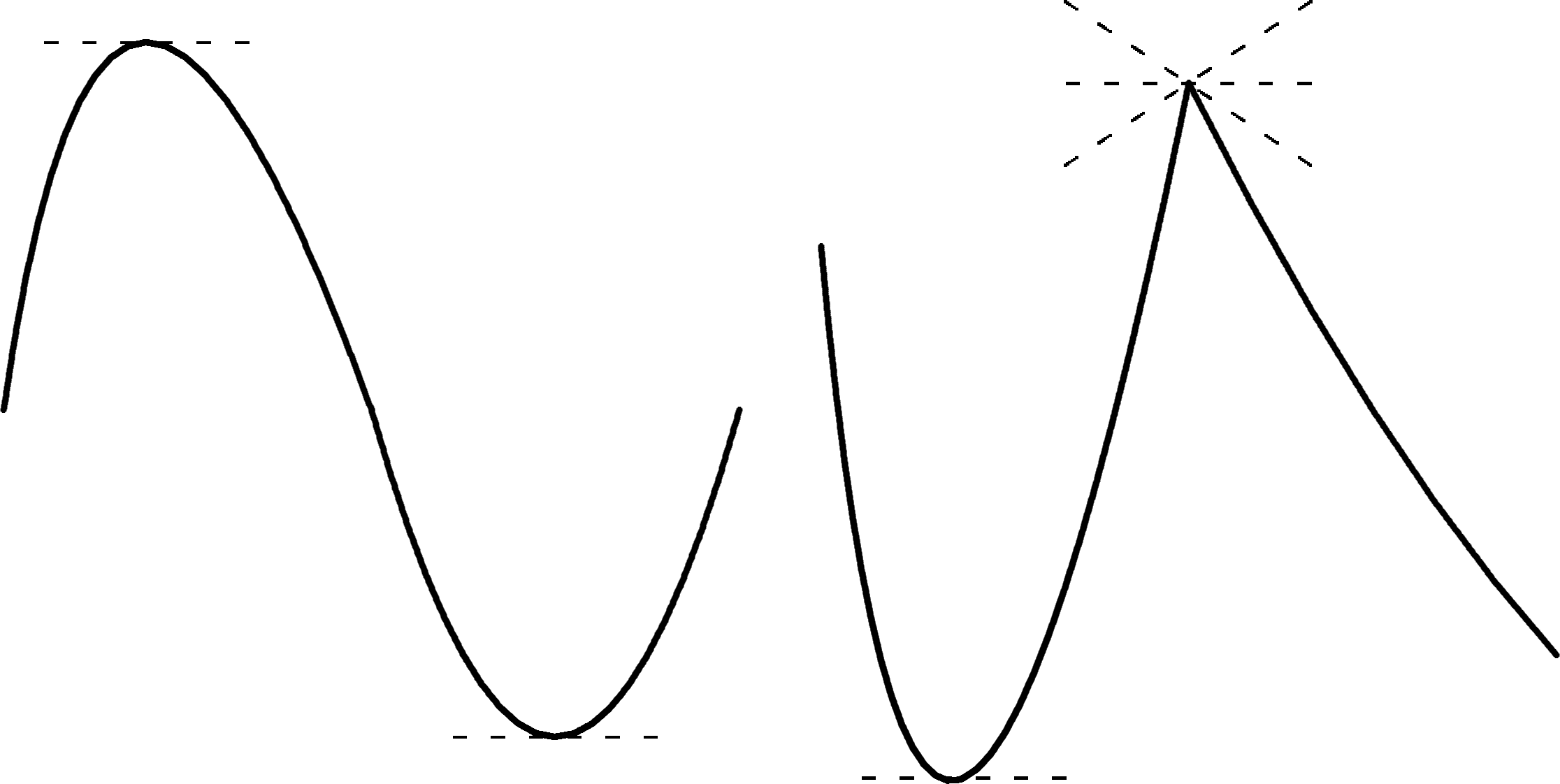
Figure 4.1: Critical points for continuous functions of a single real variable.
If additionally \(f\) is continuous, then the optimal solution of the problem \[\begin{array}{|rl} \max & f(x) \\ \text{s.t.} & x\leq b \\ & x\geq a \\ &x \in \mathbb{R} \end{array}\] is found at one (or possibly, many) of the following feasible solutions: \(x=a\), \(x=b\), or \(x=x^*\) where \(x^*\) is a critical point of \(f\) in \((a,b)\).
This can be extended fairly easily to multi-dimensional domains, with the following result.
Theorem let \(f:\mathcal{A}\subseteq \mathbb{R}^n\to \mathbb{R}\) be a continuous function, where \(\mathcal{A}\) is a closed subset of \(\mathbb{R}^n\). Then \(f\) reaches its maximum (resp.minimum) value either at a critical point of \(f\) in the interior of \(\mathcal{A}\), or somewhere on \(\partial\!\!\mathcal{A}\), the boundary of \(\mathcal{A}\).
Example: Consider a company that sells gadgets and gizmos. If the company’s monthly profits are expressed (in 1000$ dollars) according to \[f(x,y)=81+16xy-x^4-y^4,\] where \(x\) and \(y\) represent, respectively, the number of gadgets and gizmos sold monthly (in 10,000s of units), and if the company can produce up to 30,000 units of both gadgets and gizmos monthly, what is the optimal number of each items that the company must sell in order to maximize its monthly profits? The monthly profit function is shown in Figure 4.2.
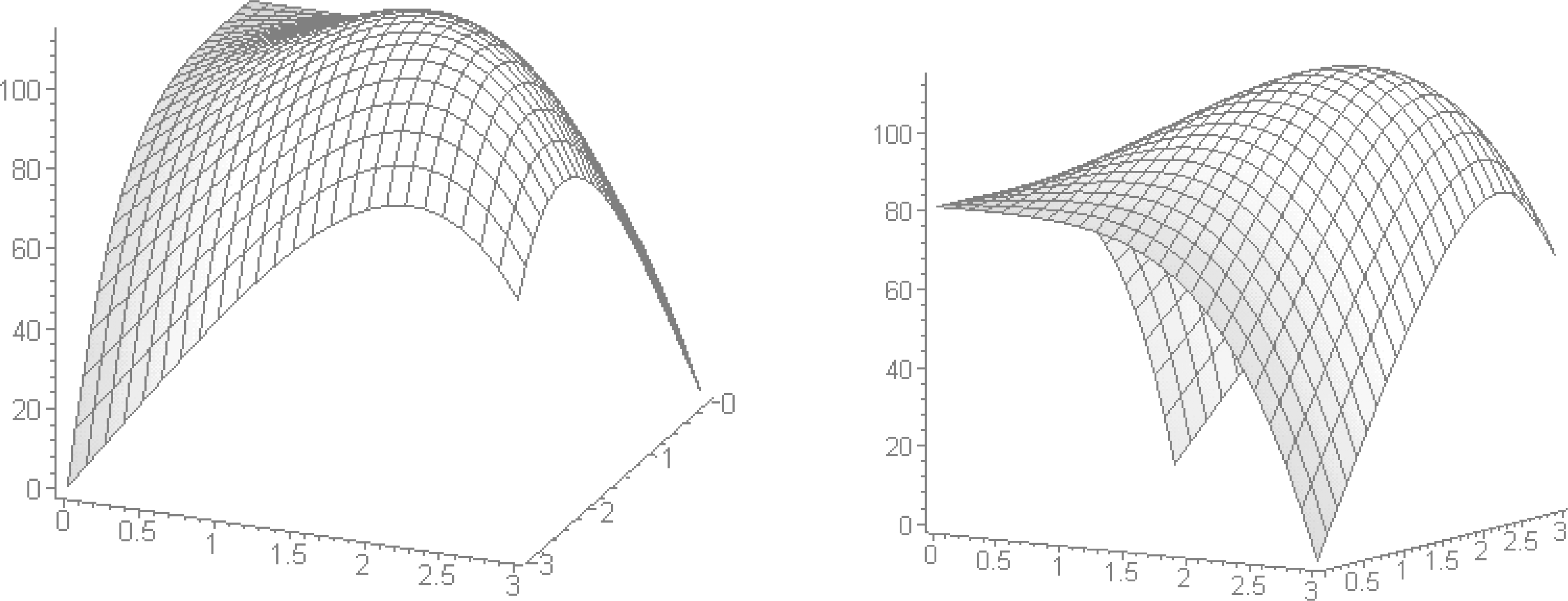
Figure 4.2: Monthly profit function for the gadgets and gizmos example.
Since \(f\) is continuous, the maximum value is reached at a critical value in \[\mathcal{A}^{\circ}=(0,3)\times (0,3)\] or somewhere on the boundary \[\partial\!\!\mathcal{A}=\{(x,y)\in [0,3]^2\mid x=0 \text{ or }x=3\text{ or }y=0\text{ or }y=3\}.\]
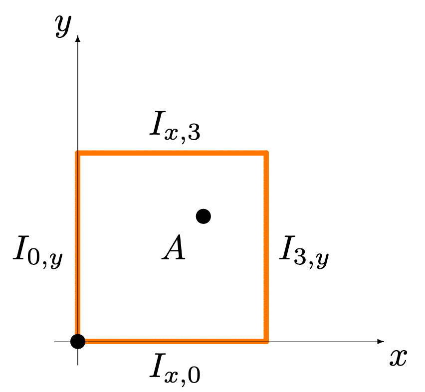
Figure 4.3: Boundary of the domain for the gadgets and gizmos example.
But \(f\) is smooth; the gradient \(\nabla f(x,y)\) is thus always defined, and the only critical points are those for which \(\nabla f(x,y)=(16y-4x^3,16x-4y^3)=(0,0)\). At such a point, \(4x=y^3\), which, upon substitution in \(f_x\) yields \[\begin{aligned} 0&=16y-\frac{1}{16}y^9=\frac{1}{16}y(256-y^8)\\&=\frac{1}{16}y(y-2)(y+2)(y^2+4)(y^4+16), \end{aligned}\] which is to say \(y=-2,0,2\).
Only \(y=2\) can potentially yield a critical point in \(\mathcal{A}^{\circ}\), however. When \(y=2\), we must have \(x=\frac{1}{4}2^3=2\): the only critical point of \(f\) in \(\mathcal{A}^{\circ}\) is thus \((x^*,y^*)=(2,2)\), and the monthly profit function value at that point is \[f(x^*,y^*)=81+16(2)(2)-2^4-2^4=113.\]
On the boundary \(\partial\!\! \mathcal{A}\), the objective function reduces to one of the following four forms: \[\begin{aligned} f(0,y)=g_0(y)&=81-y^4,\quad \text{on }0\leq y\leq 3 \\ f(3,y)=g_3(y)&=48y-y^4, \quad \text{on }0\leq y\leq 3 \\ f(x,0)=h_0(x)&=81-x^4,\quad \text{on }0\leq x\leq 3 \\ f(x,3)=h_3(x)&=48x-x^4, \quad \text{on }0\leq x\leq 3 \end{aligned}\] These are easy to optimize, being continuous functions of a single real variable; \(g_0\) and \(h_0\) are maximized at the origin, with the objective function taking the value 81 there, while \(g_3\) and \(h_3\) are maximized at \(12^{1/3}\), with the objective function taking the value \(\approx 82.42\) there (see Figure 4.4).
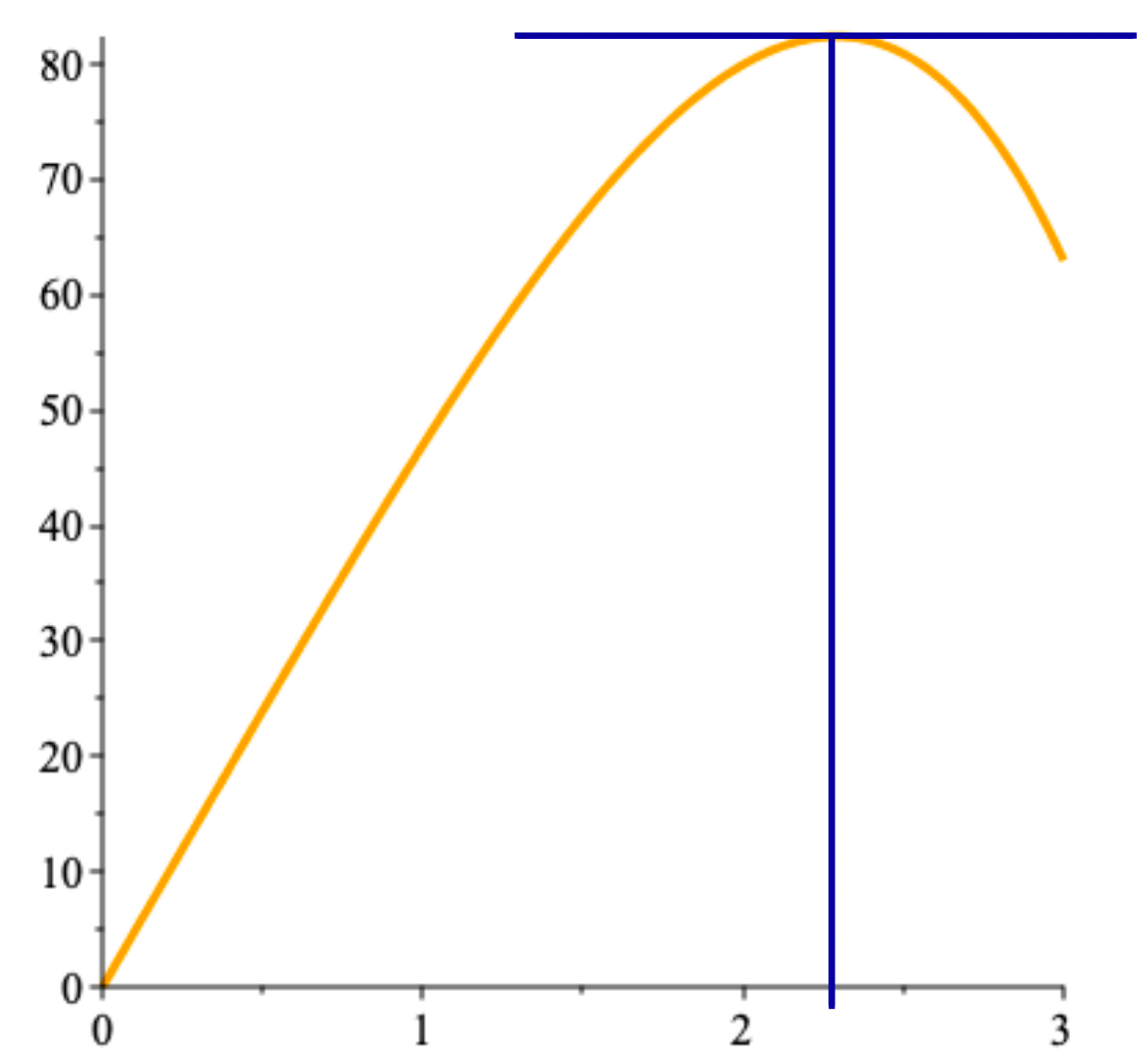
Figure 4.4: Profile for \(g_3\) and \(h_3\) in the gadgets and gizmos example.
Combining all this information, we conclude that the company will maximize its monthly profits at 113,000$ if it sells 20,000 units of both the gadgets and the gizmos.
While the approach we just presented works in this case, there are many instances for which it can be substantially more difficult to find the optimal value on \(\partial\!\!\mathcal{A}\).
The method of Lagrange multipliers can simplify the computations, to some extent. Consider the problem \[\begin{array}{|rl} \min/\max & f(\mathbf{x}) \\ \text{s.t.} & g_i(\mathbf{x})\leq a_i \quad i = 1,\ldots,m \\ & \mathbf{x} \in \mathcal{D}, \end{array}\] where \(f,g_i\) are continuous and differentiable on the (closed) region \(\mathcal{A}\) described by the constraints \(g_i\leq a_i\), \(i=1,\ldots, m\)1
If the problem is feasible and bounded, then the optimal value is reached either at a critical point of \(f\) in \(\mathcal{A}^{\circ}\) or at a point \(\mathbf{x}\in\partial\!\! \mathcal{A}\) for which \[\nabla f(\mathbf{x})=\lambda_1 \nabla g_1(\mathbf{x})+\cdots + \lambda_m\nabla g_m(\mathbf{x}),\] where \(\lambda_1,\ldots,\lambda_m\in \mathbb{R}\) are the Lagrange multipliers of the problem.
Example: consider a factory that produces various types of deluxe pickle jars. The monthly number of jars \(Q\) of a specific kind of pickled radish that can be produced at the factory is given by \(Q(K,L)=900K^{0.6}L^{0.4},\) where \(K\) is the number of dedicated canning machines, and \(L\) is the monthly number of employee-hours spent on the pickled radish.
The pay rate for the employees is 100$/hour (the pickles are extra deluxe, apparently), and the monthly maintenance cost for each canning machine is \(200\$\).
If the factory owners want to maintain monthly production at 36,000 jars of pickled radish, what combination of number of canning machines and employee-hour will minimize the total production costs? The optimization problem is \[\begin{array}{|rl} \min & f(K,L)=200K+100L \\ \text{s.t.} & K^{0.6}L^{0.4}=40 \\ & K,L \geq 0. \end{array}\]
The objective function is linear and so has no critical point. The feasability region \(\mathcal{A}\) can be described by the constraints \(g_1(K,L)=K^{0.6}L^{0.4}\leq 40\) and \(g_2(K,L)=-K^{0.6}L^{0.4}\leq -40\). Points of interest on the boundary \(\partial\!\!\mathcal{A}\) are obtained by solving the Lagrange equation \[\begin{aligned} (200,100) &=\textstyle{\lambda\left(0.6\left(\frac{L}{K}\right)^{0.4},0.4\left(\frac{K}{L}\right)^{0.6}\right)}, \end{aligned}\] since \(\nabla g_1 = -\nabla g_2\), with \(K^{0.6}L^{0.4}=40.\)
Numerically, there is only one solution, namely \[(K_*,L_*,\lambda)\approx (35.65,47.54,297.10).\] The objective function at that point takes on the value \[f(K_*,L_*)\approx 200(35.65)+100(47.54)\approx 11884.02,\] and this value must either be the maximum or the minimum of the objective function subject to the constraints of the problem.
We know, however, that the point \((K_1,L_1)= (1,40^{2.5})\) belongs to \(\partial\!\!\mathcal{A}\) (as \(1^{0.6}(40^{2.5})^{0.4}=40)\); since \[f(K_1,L_1)=200(1)+100(40^{2.5}) > f(K_*,L_*),\] then \((K_*,L_*)\) is indeed the minimal solution of the problem, and the minimal value of the objective function subject to the constraints is \(\approx 11,884.02\$\).
In practice, the value for \(K\) has to be an integer (unless we consider using a different number of canning machines at various times during the month), so we might pick:
a sub-optimal \(K'_*=36\) canning machines, which yields
a sub-optimal \(L'_*\approx 46.84\) employee-hours,
both of which yield a sub-optimal monthly operating cost of \[f(K'_*,L'_*)\approx 200(36)+100(46.84)\approx 11884.85.\]
This departure from optimality would nevertheless be quite likely to be acceptable to the factory owners.
Given how straightforward the method is, it might seem that there is no real need to say anything else – why would anybody ever use something other than Lagrange multipliers to solve optimization problems?
One of the issues is that when the number of constraints is too high relative to the dimension of \(\mathcal{D}\), which is usually the case in real-life situations, then there may not be a finite number of candidates solutions on \(\partial \!\! \mathcal{A}\), which makes this approach useless.
The method also fails when the gradient of the constraint vanishes at some critical location.
Another difficulty that might arise is that the system of equations \[\nabla f(\mathbf{x}) = \lambda_1 \nabla g_1(\mathbf{x})+\cdots + \lambda_m\nabla g_m(\mathbf{x})\] could be ill-conditioned, or highly non-linear, and numerical solutions could be hard to obtain.
Numerical methods can also be used; we will discuss those briefly in future sections.
4.3 Classification of Optimization Problems and Types of Algorithms
The computational difficulty of optimization problems, then, depends on the properties of the domain set, constraints, and the objective function.
4.3.1 Classification
Problems without constraints are said to be unconstrained. For example, least-squares minimization in statistics can be formulated as an unconstrained problem, and so can \[\begin{array}{|rl} \min & x^2 - 3x \\ \mbox{s.t.} & x \in \mathbb{R} \end{array}\]
Problems with linear constraints \(g_i\) (i.e.linear inequalities or equalities) and a linear objective function \(f\) form an important class of problems in linear programming.
Linear programming problems are by far the easiest to solve in the sense that efficient algorithms exist both in theory and in practice. Linear programming is also the backbone for solving more complex models [1]. Convex problems are problems with a convex domain set, which is to say a set \(\mathcal{D}\) such that \[t\mathbf{x}_1+(1-t)\mathbf{x}_2\in \mathcal{D}\] for all \(\mathbf{x}_1,\mathbf{x}_2\in \mathcal{D}\) and for all \(t\in [0,1]\), and convex constraints \(g_i\) and function \(f\), which is to say, \[h(t\mathbf{x}_1+(1-t)\mathbf{x}_2)\leq th(\mathbf{x}_1)+(1-t)h(\mathbf{x}_2)\] for all \(\mathbf{x}_1,\mathbf{x}_2\in \mathcal{D}\), and for all \(t\in [0,1], h\in \{f,g_i\}.\)
Convex optimization problems have the property that every local optimum is also a global optimum. Such a property permits the development of effective algorithms that could also work well in practice. Linear programming is a special case of convex optimization.
Nonconvex problems (such as problems involving integer variables and/or nonlinear constraints that are not convex) are the hardest problems to solve. In general, nonconvex problems are NP-hard. Such problems often arise in scheduling and engineering applications. In the rest of the report, we will primarily focus on linear programming and nonconvex problems whose linear constraints \(g_i\) and objective function \(f\) are linear, but with domain set \(\mathcal{D}\subseteq \mathbb{R}^k \times \mathbb{Z}_+^{n-k}\). These problems cover a large number of applications in operations research, which are often discrete in nature. We will not discuss optimization problems that arise in statistical learning and engineering applications that are modeled as nonconvex continuous models since they require different sets of techniques and methods – more information is available in [2].
4.3.2 Algorithms
We will not go into the details of algorithms for solving the problems discussed, as consultants and analytsts are expected to be using off-the-shelf solvers for the various tasks, but it could prove useful for analysts to know of the various types of algorithms or methods that exist for solving optimization problems.
Algorithms fall into three families: heuristics, exact, and approximate methods.
Heuristics are normally quick to execute but do not provide guarantees of optimality. For example, the greedy heuristic for the Knapsack Problem is very quick but does not always return an optimal solution. In fact, no guarantee exists for the “validity” of a solution either.
Other heuristics methods include ant colony, particle swarm, and evolutionary algorithms, just to name a few. There are also heuristics that are stochastic in nature and have proof of convergence to an optimal solution. Simulated annealing and multiple random starts are such heuristics.
Unfortunately, there is no guarantee on the running time to reach optimality and there is no way to identify when one has reached an optimum point.
Exact methods return a global optimum after a finite run time.
However, most exact methods can only guarantee that constraints are approximately satisfied (though the potential violations fall below some pre-specified tolerance). It is therefore possible for the returned solutions to be infeasible for the actual problem.
There also exist exact methods that fully control the error. When using such a method, an optimum is usually given as a box guaranteed to contain an optimal solution rather than a single element.
Returning boxes rather than single elements are helpful in cases, for example, where the optimum cannot be expressed exactly as a vector of floating point numbers.
Such exact methods are used mostly in academic research and in areas such as medicine and avionics where the tolerance for errors is practically zero.
Approximate methods eventually zoom in on sub-optimal solutions, while providing a guarantee: this solution is at most \(\varepsilon\) away from the optimal solution, say.
In other words, approximate methods also provide a proof of solution quality.
4.4 Linear Programming
Linear programming (LP) was developed independently by G.B. Dantzig and L. Kantorovich in the first half of the \(20^{\textrm{th}}\) century to solve resource planning problems. Even though linear programming is insufficient for many modern-day applications in operations research, it was used extensively in economic and military contexts in the early days.
To motivate some key ideas in linear programming, we begin with a small example.
Example: A roadside stand sells lemonade and lemon juice. Each unit of lemonade requires 1 lemon and 2 litres of water to prepare, and each unit of lemon juice requires 3 lemons and 1 litre of water to prepare. Each unit of lemonade gives a profit of 3$ dollars upon selling, and each unit of lemon juice gives a profit of 2$ dollars, upon selling. With 6 lemons and 4 litres of water available, how many units of lemonade and lemon juice should be prepared in order to maximize profit?
If we let \(x\) and \(y\) denote the number of units of lemonade and lemon juice, respectively, to prepare, then the profit is the objective function, given by \(3x + 2y\)$. Note that there are a number of constraints that \(x\) and \(y\) must satisfy:
\(x\) and \(y\) should be non-negative;
the number of lemons needed to make \(x\) units of lemonade and \(y\) units of lemon juice is \(x+3y\) and cannot exceed 6;
the number of litres of water needed to make \(x\) units of lemonade and \(y\) units of lemon juice is \(2x+y\) and cannot exceed 4;
Hence, to determine the maximum profit, we need to maximize \(3x + 2y\) subject to \(x\) and \(y\) satisfying the constraints \(x + 3y \leq 6\), \(2x + y \leq 4\), \(x \geq 0\), and \(y \geq 0.\) A more compact way to write the problem is as follows: \[\begin{array}{|rrcrll} \max & 3x & + & 2y & \\ \mbox{s.t.} & x & + & 3y & \leq & 6 \\ & 2x & +& y & \leq & 4 \\ & x & & & \geq & 0 \\ & & & y & \geq & 0. \\ & x & , & y & \in & \mathbb{R}. \end{array}\] It is customary to omit the specification of the domain set in linear programming since the variables always take on real numbers. Hence, we can simply write \[\begin{array}{|rrcrll} \max & 3x & + & 2y & \\ \mbox{s.t.} & x & + & 3y & \leq & 6 \\ & 2x & +& y & \leq & 4 \\ & x & & & \geq & 0 \\ & & & y & \geq & 0. \end{array}\]
We can solve the above maximization problem graphically, as follows. We first sketch the set of \([x, y]^{\!\top}\) satisfying the constraints, called the feasible region, on the \((x,y)\)-plane.
We then take the objective function \(3x+2y\) and turn it into the equation of a line \(3x+2y = c\) where \(c\) is a parameter. Note that as the value of \(c\) increases, the line defined by the equation \(3x+2y=c\) moves in the direction of the normal vector \([3,2]^{\!\top}\). We call this direction the direction of improvement. Determining the maximum value of the objective function, called the optimal value, subject to the contraints amounts to finding the maximum value of \(c\) so that the line defined by the equation \(3x+2y=c\) still intersects the feasible region.
Figure 4.5 shows the lines with \(c=0,4,6.8\).
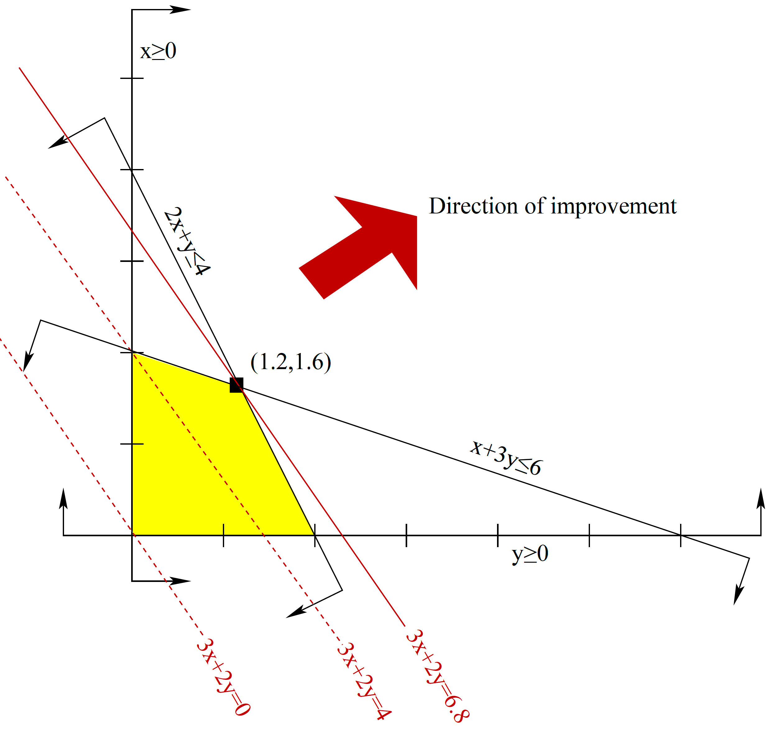
Figure 4.5: Graphical solution for the lemonade and lemon juice optimization problem; the feasible region is shown in yellow, and level curves of the objective function in red..
We can see that if \(c\) is greater than 6.8, the line defined by \(3x+2y = c\) will not intersect the feasible region. Hence, the profit cannot exceed 6.8 dollars.
As the line \(3x+2y = 6.8\) does intersect the feasible region, \(6.8\) is the maximum value for the objective function. Note that there is only one point in the feasible region that intersects the line \(3x+2y=6.8\), namely \([x^*, y^*]^{\!\top} = [ 1.2, 1.6]^{\!\top}\). In other words, to maximize profit, we want to prepare 1.2 units of lemonade and 1.6 units of lemon juice.
This solution method can hardly be regarded as rigorous because we relied on a picture to conclude that \(3x + 2y \leq 6.8\) for all \([x,y]^{\!\top}\) satisfying the constraints. But we can also obtain this result algebraically.
Note that multiplying both sides of the constraint \(x + 3y \leq 6\) by \(0.2\) yields \[0.2x + 0.6 y \leq 1.2,\] and multiplying both sides of the constraint \(2x + y \leq 4\) by \(1.4\) yields \[2.8x + 1.4 y \leq 5.6.\] Hence, any \([x,y]^{\!\top}\) that satisfies both \[x+3y\leq 6\quad\mbox{and}\quad 2x+y \leq 4\] must also satisfy \[(0.2x+0.6y) + (2.8x+1.4y) \leq 1.2 + 5.6,\] which simplifies to \(3x + 2y \leq 6.8\), as desired.
It is always possible to find an algebraic proof like the one above for linear programming problems, which adds to their appeal. To describe the full result, it is convenient to call on duality, a central notion in mathematical optimization.
4.4.1 Linear Programming Duality
Let (P) denote following linear programming problem: \[\begin{array}{|rl} \min & \mathbf{c}^\mathsf{T} \mathbf{x} \\ \mbox{s.t.} & \mathbf{A}\mathbf{x} \geq \mathbf{b} \end{array}\] where \(\mathbf{c} \in \mathbb{R}^n\) \(\mathbf{b} \in \mathbb{R}^m\) \(\mathbf{A} \in \mathbb{R}^{m\times n}\) (inequality on \(m-\)tuples is applied component-wise.)
Then for every \(\mathbf{y} \in \mathbb{R}^m_+\) (that is, all components of \(\mathbf{y}\) are non-negative), the inferred inequality \(\mathbf{y}^\mathsf{T}\mathbf{A}\mathbf{x} \geq \mathbf{y}^\mathsf{T} \mathbf{b}\) is valid for all \(\mathbf{x}\) satisfying \(\mathbf{A}\mathbf{x} \geq \mathbf{b}\).
Furthermore, if \(\mathbf{y}^\mathsf{T}\mathbf{A} = \mathbf{c}^\mathsf{T},\) the inferred inequality becomes \(\mathbf{c}^\mathsf{T} \mathbf{x} \geq \mathbf{y}^\mathsf{T} \mathbf{b}\), making \(\mathbf{y}^\mathsf{T} \mathbf{b}\) a lower bound on the optimal value of (P). To obtain the largest possible bound, we can solve \[\begin{array}{|rl} \max & \mathbf{y}^\mathsf{T} \mathbf{b} \\ \mbox{s.t.} & \mathbf{y}^\mathsf{T} \mathbf{A} = \mathbf{c}^\mathsf{T} \\ & \mathbf{y} \geq \mathbf{0}. \end{array}\]
This problem is called the dual problem of (P), and (P) is called the primal problem. A remarkable result relating (P) and its dual (P’) is the Duality Theorem for Linear Programming: if (P) has an optimal solution, then so does its dual problem (P’), and the optimal values of the two problems are the same.
A weaker result follows easily from the discussion above: the objective function value of a feasible solution to the dual problem (P’) is a lower bound on the objective function value of a feasible solution to (P). This result is known as weak duality. Despite the fact that it is a simple result, its significance in practice cannot be overlooked because it provides a way to gauge the quality of a feasible solution to (P).
For example, suppose we have at hand a feasible solution to (P) with objective function value 3 and a feasible solution to the dual problem (P’) with objective function value 2. Then we know that the objective function value of our current solution to (P) is within \(1.5\) times the actual optimal value since the optimal value cannot be less than \(2\).
In general, a linear programming problem can have a more complicated form. Let \(\mathbf{A} \in \mathbb{R}^{m\times n}\), \(\mathbf{b} \in \mathbb{R}^m\), \(\mathbf{c} \in \mathbb{R}^n\). Let \({\mathbf{a}^{(i)}}^\mathsf{T}\) denote the \(i\)th row of \(\mathbf{A}\), \(\mathbf{A}_j\) denote the \(j\)th column of \(\mathbf{A}\), and (P) denote the minimization problem, with variables in the tuple \(\mathbf{x} = [ x_1, \cdots, x_n]^{\!\top}\), given as follows:
the objective function to be minimized is \(\mathbf{c}^\mathsf{T} \mathbf{x}\);
the constraints are \({\mathbf{a}^{(i)}}^\mathsf{T}\mathbf{x}~\sqcup_i~b_i\), where \(\sqcup_i\) is \(\leq\), \(\geq\), or \(=\) for \(i = 1,\ldots, m\), and
for each \(j \in \{1,\ldots,n\}\), \(x_j\) is constrained to be non-negative, nonpositive, or free.
Then the dual problem (P’) is defined to be the maximization problem, with variables in the tuple \(\mathbf{y} = [ y_1, \cdots, y_m]^{\!\top}\) given as follows:
the objective function to be maximized is \(\mathbf{y}^\mathsf{T} \mathbf{b}\);
for \(j = 1,\ldots, n\), the \(j\)th constraint is \[\left \{\begin{array}{ll} \mathbf{y}^\mathsf{T}\mathbf{A}_j \leq c_j & \text{if } x_j \text{ is constrained to be non-negative} \\ \mathbf{y}^\mathsf{T}\mathbf{A}_j \geq c_j & \text{if } x_j \text{ is constrained to be nonpositive} \\ \mathbf{y}^\mathsf{T}\mathbf{A}_j = c_j & \text{if } x_j \text{ is free}. \end{array}\right.\]
and for each \(i \in \{1,\ldots,m\}\), \(y_i\) is constrained to be non-negative if \(\sqcup_i\) is \(\geq\); \(y_i\) is constrained to be non-positive if \(\sqcup_i\) is \(\leq\); \(y_i\) is free if \(\sqcup_i\) is \(=\).
The following table can help remember the correspondences:
| Primal (min) | Dual (max) |
|---|---|
| \(\geq\) constraint | \(\geq 0\) variable |
| \(\leq\) constraint | \(\leq 0\) variable |
| \(=\) constraint | free variable |
| \(\geq 0\) variable | \(\geq\) constraint |
| \(\leq 0\) variable | \(\leq\) constraint |
| free variable | \(=\) constraint |
Below is an example of a primal-dual pair of problems based on the above definition.
Consider the primal problem: \[\begin{array}{|rrcrcrcl} \mbox{min} & x_1 & - & 2x_2 & + & 3x_3 & \\ \mbox{s.t.} & -x_1 & & & + & 4x_3 & = &5 \\ & 2x_1 & + & 3x_2 & - & 5x_3 & \geq & 6 \\ & & & 7x_2 & & & \leq & 8 \\ & x_1 & & & & & \geq & 0 \\ & & & x_2 & & & & \mbox{free} \\ & & & & & x_3 & \leq & 0.\\ \end{array}\] Here, \(\mathbf{A}= \begin{bmatrix} -1 & 0 & 4 \\ 2 & 3 & -5 \\ 0 & 7 & 0 \end{bmatrix}\), \(\mathbf{b} = \begin{bmatrix}5 \\6\\8\end{bmatrix}\), and \(\mathbf{c} = \begin{bmatrix}1 \\-2\\3\end{bmatrix}\).
Since the primal problem has three constraints, the dual problem has three variables:
the first constraint in the primal is an equation, the corresponding variable in the dual is free;
the second constraint in the primal is a \(\geq\)-inequality, the corresponding variable in the dual is non-negative;
the third constraint in the primal is a \(\leq\)-inequality, the corresponding variable in the dual is non-positive.
Since the primal problem has three variables, the dual problem has three constraints:
the first variable in the primal is non-negative, the corresponding constraint in the dual is a \(\leq\)-inequality;
the second variable in the primal is free, the corresponding constraint in the dual is an equation;
the third variable in the primal is non-positive, the corresponding constraint in the dual is a \(\geq\)-inequality.
Hence, the dual problem is: \[\begin{array}{|rrcrcrcl} \max & 5y_1 & + & 6y_2 & + & 8y_3 & \\ \mbox{s.t.} & -y_1 & + & 2y_2 & & & \leq & 1 \\ & & & 3y_2 & + & 7y_3 & = & -2 \\ & 4y_1 & - & 5y_2 & & & \geq & 3 \\ & y_1 & & & & & & \mbox{free} \\ & & & y_2 & & & \geq & 0 \\ & & & & & y_3 & \leq & 0.\\ \end{array}\]
In some references, the primal problem is always a maximization problem – in that case, what we have considered to be a primal problem is their dual problem and vice-versa.
Note that the Duality Theorem for Linear Programming remains true for the more general definition of the primal-dual pair of linearprogramming problems.
4.4.2 Methods for Solving Linear Programming Problems
There are currently two families of methods used by modern-day linear programming solvers: simplex methods and interior-point methods.
We will not get into the technical details of these methods, except to say that the algorithms in either family are iterative, that there is no known simplex method that runs in polynomial time, but efficient polynomial-time interior-point methods abound in practice. We might wonder why anyone would still use simplex methods, given that they are not polynomial-time methods: simply put, simplex methods are in general more memory-efficient than interior-point methods, and they tend to return solutions that have few nonzero entries.
More concretely, suppose that we want to solve the following problem: \[\begin{array}{|rl} \min & \mathbf{c}^\mathsf{T}\mathbf{x} \\ \mbox{s.t.} & \mathbf{A}\mathbf{x} = \mathbf{b} \\ & \mathbf{x} \geq \mathbf{0}. \end{array}\]
For ease of exposition, we assume that \(\mathbf{A}\) has full row rank. Then, each iteration of a simplex method maintains a current solution \(\mathbf{x}\) that is basic, in the sense that the columns of \(\mathbf{A}\) corresponding to the nonzero entries of \(\mathbf{x}\) are linearly independent. In contrast, interior-point methods will maintain \(\mathbf{x} > \mathbf{0}\) throughout (whence the name “interior point”).
When we use an off-the-shelf linear programming solver, the choice of method is usually not too important since solvers have good default settings. Simplex methods are typically used in settings when a problem needs to be resolved after minor changes in the problem data or in problems with additional integrality constraints discussed in the next section.
4.5 Mixed-Integer Linear Programming
While the simplicity of linear programming (and duality) make it an appealing tool, its modeling power is insufficient in many real-life applications (for example, there is no simple linear programming formulation of the BKP).
Fortunately, allowing the domain set to restrict one or more variables to integer values drastically extends the modeling power. The price we pay is that there is no guarantee that the problems can be solved in polynomial time.
Example: Recall the lemonade and lemon juice problem introduced in the previous section: there is a unique optimal solution at \([x,y]^{\!\top} = [ 1.2 , 1.6]^{\!\top}\) for a profit of \(6.8\).
But this solution requires the preparation of fractional units of lemonade and lemon juice. What if the number of prepared units needs to be integers?
The solution is to add integrality constraints: \[\begin{array}{|rrcrll} \max & 3x & + & 2y & \\ \text{s.t.} & x & + & 3y & \leq & 6 \\ & 2x & +& y & \leq & 4 \\ & x & & & \geq & 0 \\ & & & y & \geq & 0 \\ & x &,& y & \in & \mathbb{Z}. \\ \end{array}\]
This problem is no longer a linear programming problem; rather, it is an integer linear programming problem. Note that we can solve this problem via a case analysis. The second and third inequalities tell us that the possible values for \(x\) are \(0\), \(1\), and \(2\).
If \(x = 0\), the first inequality gives \(3y \leq 6\), implying that \(y \leq 2\). Since we are maximizing \(3x+2y\), we want \(y\) to be as large as possible; \([x,y ]^{\!\top} = [ 0,2 ]^{\!\top}\) satisfies all the constraints with an objective function value of \(4\).
If \(x = 1\), the first inequality gives \(3y \leq 5\), implying that \(y \leq 1\). Note that \([x, y ]^{\!\top} = [ 1, 1 ]^{\!\top}\) satisfies all the constraints with an objective function value of \(5\).
If \(x = 2\), the second inequality gives \(y \leq 0\). Note that \([x, y ]^{\!\top} = [ 2, 0 ]^{\!\top}\) satisfies all the constraints with an objective function value of \(6\).
Thus, \([x^*,y^* ]^{\!\top} = [ 2,0 ]^{\!\top}\) is an optimal solution. How does this compare to the solution of the LP problem of the previous section, both in terms of location of the solution and value of the objective function?
A mixed-integer linear programming problem (MILP) is a problem of minimizing or maximizing a linear function subject to finitely many linear constraints such that the number of variables are finite, with at least one of them required to take on integer values.
If all the variables are required to take on integer values, the problem is called a pure integer linear programming problem or simply an integer linear programming problem. Normally, we assume the problem data to be rational numbers to rule out pathological cases.
Many solution methods for solving MILPs have been devised and some of them first solve the linear programming relaxation of the original problem, which is the problem obtained from the original problem by dropping all the integrality requirements on the variables.
For instance, if (MP) denotes the following mixed-integer linear programming problem: \[\begin{array}{|rrcrcrlll} \min & x_1 & & & + & x_3 \\ \mbox{s.t.} & -x_1 & + & x_2 & + & x_3 & \geq & 1 \\ & -x_1 & - & x_2 & + & 2x_3 & \geq & 0 \\ & -x_1 & + & 5x_2 & - & x_3 & = & 3 \\ & x_1 & , & x_2 & , & x_3 & \geq & 0 \\ & & & & & x_3 & \in & \mathbb{Z}. \end{array}\] then the linear programming relaxation (P1) of (MP) is: \[\begin{array}{|rrcrcrlll} \mbox{min} & x_1 & & & + & x_3 \\ \text{s.t.} & -x_1 & + & x_2 & + & x_3 & \geq & 1 \\ & -x_1 & - & x_2 & + & 2x_3 & \geq & 0 \\ & -x_1 & + & 5x_2 & - & x_3 & = & 3 \\ & x_1 & , & x_2 & , & x_3 & \geq & 0. \end{array}\]
Observe that the optimal value of (P1) is a lower bound for the optimal value of (MP) since the feasible region of (P1) contains all the feasible solutions to (MP), thus making it possible to find a feasible solution to (P1) with objective function value which is better than the optimal value of (MP).
Hence, if an optimal solution to the linear programming relaxation happens to be a feasible solution to the original problem, then it is also an optimal solution to the original problem. Otherwise, there is an integer variable having a nonintegral value \(v\).
What we then do is to create two new sub-problems as follows:
one requiring the variable to be at most the greatest integer less than \(v\),
the other requiring the variable to be at least the smallest integer greater than \(v\).
This is the basic idea behind the branch-and-bound method. We now illustrate these ideas on (MP). Solving the linear programming relaxation (P1), we find that \(\mathbf{x}' = \frac{1}{3}[0,2,1]^{\!\top}\) is an optimal solution to (P1). Note that \(\mathbf{x}'\) is not a feasible solution to (MP) because \(x'_3\) is not an integer. We now create two sub-problems (P2) and (P3).
(P2) is obtained from (P1) by adding the constraint \[x_3 \leq \lfloor x'_3\rfloor\] and (P3) is obtained from (P1) by adding the constraint \[x_3 \geq \lceil x'_3\rceil.\footnote{\(\lfloor a \rfloor\) denotes the \textbf{floor of} \(a\) and \(\lceil a \rceil\) denotes the \textbf{ceiling of} \(a\).}\] Hence, (P2) is the problem \[\begin{array}{|rrcrcrlll} \min & x_1 & & & + & x_3 \\ \text{s.t.} & -x_1 & + & x_2 & + & x_3 & \geq & 1 \\ & -x_1 & - & x_2 & + & 2x_3 & \geq & 0 \\ & -x_1 & + & 5x_2 & - & x_3 & = & 3 \\ & & & & & x_3 & \leq & 0 \\ & x_1 & , & x_2 & , & x_3 & \geq & 0, \end{array}\] and (P3) is the problem \[\begin{array}{|rrcrcrlll} \min & x_1 & & & + & x_3 \\ \text{s.t.} & -x_1 & + & x_2 & + & x_3 & \geq & 1 \\ & -x_1 & - & x_2 & + & 2x_3 & \geq & 0 \\ & -x_1 & + & 5x_2 & - & x_3 & = & 3 \\ & & & & & x_3 & \geq & 1 \\ & x_1 & , & x_2 & , & x_3 & \geq & 0. \end{array}\]
Note that any feasible solution to (MP) must be a feasible solution to either (P2) or (P3). Using the help of a solver, one can see that (P2) is infeasible. The problem (P3), however, has an optimal solution at \(\mathbf{x}^* = \frac{1}{5}[0,4,5]^{\!\top}\), which is also feasible for (MP). Hence, \(\mathbf{x}^*\) is an optimal solution of (MP).
In many instances, there are multiple choices for the variable on which to branch, and for which sub-problem to solve next. These choices can have an impact on the total computation time. Unfortunately, there are no hard-and-fast rules at the moment to determine the best branching path. This in area of ongoing research.
4.5.1 Cutting Planes
Difficult MILP problems often cannot be solved by branch-and-bound methods alone. A technique that is typically employed in solvers is to add valid inequalities to strengthen the linear programming relaxation.
Such inequalities, known as cutting planes, are known to be satisfied by all the feasible solutions to the original problem but not by all the feasible solutions to the initial linear programming relaxation.
Example: consider the following PILP problem: \[\begin{array}{|rrcrlll} \min & 3x & + & 2y \\ \text{s.t.} & 2x & + & y & \geq & 1 \\ & x & + & 2y & \geq & 4 \\ & x & , & y & \in & \mathbb{Z}. \end{array}\]
An optimal solution to the linear programming relaxation is given by \[[x^+, y^+ ]^{\!\top} = \frac{1}{3}[ -2,7 ]^{\!\top}.\] Note that adding the inequalities \(2x + y \geq 1\) and \(x + 2y \geq 4\) yields \(3x + 3y \geq 5\), or equivalently, \[x + y \geq \frac{5}{3}.\] Since \(x+y\) is an integer for every feasible solution \([x,y ]^{\!\top}\), \(x + y \geq 2\) is a valid inequality for the original problem, but is violated by \([x^+, y^+ ]^{\!\top}\). Hence, \(x + y \geq 2\) is a cutting plane.
Adding this to the linear programming relaxation, we have \[\begin{array}{|rrcrlll} \min & 3x & + & 2y \\ \text{s.t.} & 2x & + & y & \geq & 1 \\ & x & + & 2y & \geq & 4 \\ & x & + & y & \geq & 2. \end{array}\] which, upon solving, yields \([x^*,y^* ]^{\!\top} = [ -1,3 ]^{\!\top}\) as an optimal solution.
Since all the entries are integers, this is also an optimal solution to the original problem. In this example, adding a single cutting plane solved the problem. In practice, one often needs to add numerous cutting planes and then continue with branch-and-bound to solve nontrivial MILP problems.
Many methods for generating cutting planes exist – the problem of generating effective cutting planes efficiently is still an active area of research [3].
4.6 A Sample of Useful Modeling Techniques
So far, we have discussed the kinds of optimization problems that can be solved and certain methods available for solving them. Practical success, however, depends upon the effective translation and formulation of a problem description into a mathematical programming problem, which often turns out to be as much an art as it is a science.
We will not be discussing formulation techniques in detail (see [4] for a deep dive into the topic) – instead, we highlight modeling techniques that often arise in business applications, which our examples have not covered so far.
4.6.1 Activation
Sometimes, we may want to set a binary variable \(y\) to 1 whenever some other variable \(x\) is positive. Assuming that \(x\) is bounded above by \(M\), the inequality \[x \leq My\] will model the condition. Note that if there is no valid upper bound on \(x\), the condition cannot be modeled using a linear constraint.
4.6.2 Disjunction
Sometimes, we want \(\mathbf{x}\) to satisfy at least one of a list of inequalities; that is, \[{\mathbf{a}^{(1)}}^\mathsf{T}\mathbf{x} \geq b_1 \lor {\mathbf{a}^{(2)}}^\mathsf{T}\mathbf{x} \geq b_2 \lor \cdots \lor {\mathbf{a}^{(k)}}^\mathsf{T}\mathbf{x} \geq b_k.\] To formulate such a disjunction using linear constraints, we assume that, for \(i = 1,\ldots,k\), there is a lower bound \(M_i\) on \({\mathbf{a}^i}^\mathsf{T}\mathbf{x}\) for all \(\mathbf{x}\in \mathcal{D}\). Note that such bounds automatically exist when \(\mathcal{D}\) is a bounded set, which is often the case in applications.
The disjunction can now be formulated as the following system where \(y_i\) is a new 0-1 variable for \(i = 1,\ldots,k\): \[\begin{array}{|l} {\mathbf{a}^{(1)}}^\mathsf{T}\mathbf{x} \geq b_1 y_1 + M_1(1-y_1) \\ {\mathbf{a}^{(2)}}^\mathsf{T}\mathbf{x} \geq b_2 y_2 + M_2(1-y_2) \\ \qquad\quad \vdots \\ {\mathbf{a}^{(k)}}^\mathsf{T}\mathbf{x} \geq b_k y_k + M_k(1-y_k) \\ y_1 + \cdots + y_k \geq 1. \end{array}\]
Note that \({\mathbf{a}^i}^\mathsf{T}\mathbf{x} \geq b_i y_i + M_i(1-y_i)\) reduces to \({\mathbf{a}^i}^\mathsf{T}\mathbf{x} \geq b_i\) when \(y_i = 1\), and to \({\mathbf{a}^i}^\mathsf{T}\mathbf{x} \geq M_i\) when \(y_i = 0\), which holds for all \(\mathbf{x} \in \mathcal{D}.\)
Therefore, \(y_i\) is an activation for the \(i^{\textrm{th}}\) constraint, and at least one is activated because of the constraint \[y_1 + \cdots + y_k \geq 1.\]
4.6.3 Soft Constraints
Sometimes, we may be willing to pay a price in exchange for specific constraints to be violated (perhaps they represent “nice-to-have” conditions instead of “must-be-met” conditions). Such constraints are referred to as soft constraints.
There are situations in which having soft constraints is advisable, say when enforcing all constraints results into an infeasible problem, but a solution is nonetheless needed.
We illustrate the idea on a modified BKP. As usual, there are \(n\) items and item \(i\) has weight \(w_i\) and value \(v_i>0\) for \(i = 1,\ldots, n\). The capacity of the knapsack is denoted by \(K\). Suppose that we prefer not to take more than \(N\) items, but that the preference is not an actual constraint.
We assign a penalty for its violation and use the following formulation: \[\begin{array}{|rl} \max & \sum\limits_{i = 1}^n v_i x_i - p y\\ \mbox{s.t.} & \sum\limits_{i = 1}^n w_i x_i \leq K \\ & \sum\limits_{i = 1}^n x_i - y \leq N \\ & x_i \in \{0,1\} \quad i = 1,\ldots, n \\ & y \geq 0. \end{array}\]
Here, \(p\) is a non-negative number of our choosing. As we are maximizing \[\sum\limits_{i = 1}^n v_i x_i - p y,\] \(y\) is pushed towards 0 when \(p\) is relatively large. Therefore, the problem will be biased towards solutions that try to violate \(x_1+\cdots+x_n \leq N\) as little as possible.
Experimentation is required to determine What value to select for \(p\); the general rule is that if violation is costly in practice, we should set \(p\) to be (relatively) high; otherwise, we set it to a moderate value relative to the coefficients of the variables in the objective function value.
Note that when \(p=0\) , the constraint \(x_1+\cdots+x_n \leq N\) has no effect because \(y\) can take on any positive value without incurring a penalty.
4.7 Software Solvers
A wide variety of solvers exist for all kinds of optimization problems. The NEOS Server is a free online service that hosts many solvers and is a great resource for experimenting with different solvers on small problems.
For large or computationally challenging problems, it is advisable to use a solver installed on a dedicated private machine/server. Commercial solvers can also prove useful:
There are popular open-source solvers as well, although they are not as powerful as the commercial tools:
We mention in passing that learning how to use of any of these solvers effectively requires a significant time investment. In addition, it is common to build optimization models using a modeling system such as GAMS and LINDO, or a modeling language such as AMPL, ZIMPL, or JuMP.
Note that in the data science and machine learning context, more straightforward methods like gradient descent, stochastic gradient descent and Newton’s method are usually sufficient for most applications.
References
[1] D. Bertsimas and J. Tsitsiklis, Introduction to linear optimization, 1st ed. Athena Scientific, 1997.
[2] D. P. Bertsekas, Nonlinear programming. Athena Scientific, 1999.
[3] G. Cornuéjols, “Valid inequalities for mixed integer linear programs.” Math. Program., vol. 112, no. 1, pp. 3–44, Mar. 2008,Available: http://dblp.uni-trier.de/db/journals/mp/mp112.html#Cornuejols08
[4] H. P. Williams, “Model building in linear and integer programming,” in Computational mathematical programming, 1985, pp. 25–53.
Strictly speaking, differentiability is not required on the entirety of \(\mathcal{A}\).↩︎