Singular Value Decomposition - Properties of Symmetric Matrices 2

Geometrical interpretation of eigendecomposition ¶

In the previous post, we showed how to express a symmetric matrix as the product of three matrices, a process known as eigendecomposition. In this post, we revisit this procedure, but from a geometrical perspective.

To begin, let’s assume that a symmetric matrix $\mathbf{A}$ has $n$ eigenvectors, and each eigenvector ${\mathbf{u}}_i$ is an $n\times 1$ column vector

$${\mathbf{u}}_i=\left[\begin{array}{c}{u}_{i1}\\ u_{i2}\\ ⋮\\ u_{in}\end{array}\right]$$

then the transpose of ${\mathbf{u}}_i$ is a $1\times n$ row vector

$${\mathbf{u}}_i^T=\left[\begin{array}{cccc}{u}_{i1}& u_{i2}& \dots & u_{in}\end{array}\right]$$

and their multiplication

$${\mathbf{u}}_i{\mathbf{u}}_i^T=\left[\begin{array}{c}{u}_{i1}\\ u_{i2}\\ ⋮\\ u_{in}\end{array}\right]\left[\begin{array}{cccc}{u}_{i1}& u_{i2}& \dots & u_{in}\end{array}\right]=\left[\begin{array}{cccc}{u}_{i1}{u}_{i1}& u_{i1}{u}_{i2}& \dots & u_{in}{u}_{in}\\ u_{i2}{u}_{i1}& u_{i2}{u}_{i2}& \dots & u_{i2}{u}_{in}\\ ⋮& ⋮& ⋮& ⋮\\ u_{in}{u}_{i1}& u_{in}{u}_{i2}& \dots & u_{in}{u}_{in}\end{array}\right]$$

becomes an $n\times n$ matrix.

Let’s return to $\mathbf{A}=\mathbf{P}\mathbf{D}{\mathbf{P}}^{\mathrm{\top }}$. First, we calculate $\mathbf{D}{\mathbf{P}}^{\mathrm{\top }}$ to simplify the eigendecomposition equation:

$$\begin{array}{rl}\left[\begin{array}{cccc}{\lambda }_1& 0& \dots & 0\\ 0& {\lambda }_2& \dots & 0\\ ⋮& ⋮& ⋮& ⋮\\ 0& 0& \dots & {\lambda }_n\end{array}\right]\left[\begin{array}{c}{\mathbf{u}}_1^{\mathrm{\top }}\\ {\mathbf{u}}_2^{\mathrm{\top }}\\ \dots \\ {\mathbf{u}}_n^{\mathrm{\top }}\end{array}\right]& =\left[\begin{array}{cccc}{\lambda }_1& 0& \dots & 0\\ 0& {\lambda }_2& \dots & 0\\ ⋮& ⋮& ⋮& ⋮\\ 0& 0& \dots & {\lambda }_n\end{array}\right]\left[\begin{array}{cccc}{u}_{11}& u_{12}& \dots & u_{1n}\\ u_{21}& u_{22}& \dots & u_{2n}\\ ⋮& ⋮& ⋮& ⋮\\ u_{n1}& u_{n2}& \dots & u_{nn}\end{array}\right]\\ & =\left[\begin{array}{cccc}{\lambda }_1{u}_{11}& {\lambda }_1{u}_{12}& \dots & {\lambda }_1{u}_{1n}\\ {\lambda }_2{u}_{21}& {\lambda }_2{u}_{22}& \dots & {\lambda }_2{u}_{2n}\\ ⋮& ⋮& ⋮& ⋮\\ {\lambda }_n{u}_{n1}& {\lambda }_n{u}_{n2}& \dots & {\lambda }_n{u}_{nn}\end{array}\right]=\left[\begin{array}{c}{\lambda }_1{\mathbf{u}}_1^{\mathrm{\top }}\\ {\lambda }_2{\mathbf{u}}_2^{\mathrm{\top }}\\ \dots \\ {\lambda }_n{\mathbf{u}}_n^{\mathrm{\top }}\end{array}\right]\end{array}$$

Now the eigendecomposition becomes:

$$\mathbf{A}=\left[\begin{array}{cccc}{\mathbf{u}}_1& {\mathbf{u}}_2& \cdots & {\mathbf{u}}_n\end{array}\right]\left[\begin{array}{c}{\lambda }_1{\mathbf{u}}_1^{\mathrm{\top }}\\ {\lambda }_2{\mathbf{u}}_2^{\mathrm{\top }}\\ \dots \\ {\lambda }_n{\mathbf{u}}_n^{\mathrm{\top }}\end{array}\right]={\lambda }_1{\mathbf{u}}_1{\mathbf{u}}_1^{\mathrm{\top }}+{\lambda }_2{\mathbf{u}}_2{\mathbf{u}}_2^{\mathrm{\top }}+\dots +{\lambda }_n{\mathbf{u}}_n{\mathbf{u}}_n^{\mathrm{\top }}$$

Therefore, the $n\times n$ matrix $\mathbf{A}$ can be broken into $n$ matrices with the same shape ($n\times n$), and each of these matrices has a multiplier which is equal to the corresponding eigenvalue ${\lambda }_i$. Each of the matrices ${\mathbf{u}}_i{\mathbf{u}}_i^{\mathrm{\top }}$ is called a projection matrix.

Imagine that we have a vector $\mathbf{x}$ and a unit vector $\mathbf{v}$. The inner product of $\mathbf{v}$ and $\mathbf{x}$ which is equal to $\mathbf{v}\cdot \mathbf{x}={\mathbf{v}}^{\mathrm{\top }}\mathbf{x}$ gives the scalar projection of $\mathbf{x}$ onto $\mathbf{v}$, which is the length of the vector projection of $\mathbf{x}$ into $\mathbf{v}$. If we multiply ${\mathbf{v}}^{\mathrm{\top }}\mathbf{x}$ by $\mathbf{v}$ again, $\mathbf{v}{\mathbf{v}}^{\mathrm{\top }}\mathbf{x}$ gives a vector which is called the orthogonal projection of $\mathbf{x}$ onto $\mathbf{v}$. This is shown in Figure 1.

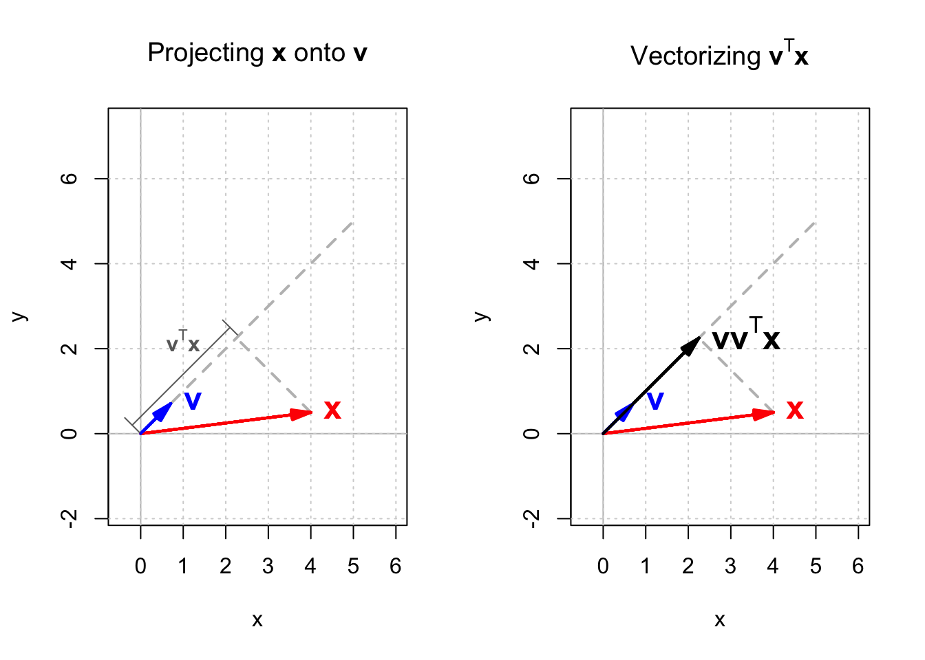
Therefore, when $\mathbf{v}$ is a unit vector, multiplying $\mathbf{v}{\mathbf{v}}^{\mathrm{\top }}$ by $\mathbf{x}$ will give the orthogonal projection of $\mathbf{x}$ onto $\mathbf{v}$, and that is why $\mathbf{v}{\mathbf{v}}^{\mathrm{\top }}$ is called the projection matrix. Multiplying ${\mathbf{u}}_i{\mathbf{u}}_i^{\mathrm{\top }}$ by $\mathbf{x}$, we get the orthogonal projection of $\mathbf{x}$ onto ${\mathbf{u}}_i$.

Now let’s use R to calculate the projection matrices of matrix $\mathbf{A}$ mentioned before.

$$\mathbf{A}=\left[\begin{array}{cc}3& 1\\ 1& 2\end{array}\right]$$

We had already calculated the eigenvalues and eigenvectors of $\mathbf{A}$.

mat_a <- matrix(c(3, 1, 1, 2), 2)
eigen_a <- eigen(mat_a)
eigen_a

eigen() decomposition
$values
[1] 3.618034 1.381966

$vectors
           [,1]       [,2]
[1,] -0.8506508  0.5257311
[2,] -0.5257311 -0.8506508

The next chunk will apply eigendecomposition to $\mathbf{A}$ and print the first term, namely ${\mathbf{A}}_1$.

u_a <- eigen_a$vectors # an orthogonal matrix made of A's eigenvectors
lambda_a <- eigen_a$values # a vector of A's eigenvalues
mat_a1 <- lambda_a[1] * u_a[,1] %*% t(u_a[,1])
mat_a1 |> round(3)

      [,1]  [,2]
[1,] 2.618 1.618
[2,] 1.618 1.000

$$\begin{array}{rl}{\mathbf{A}}_1& ={\lambda }_1{\mathbf{u}}_1{\mathbf{u}}_1^{\mathrm{\top }}\\ & =3.618\left[\begin{array}{c}-0.851\\ -0.526\end{array}\right]\left[\begin{array}{cc}-0.851& -0.526\end{array}\right]=\left[\begin{array}{cc}2.618& 1.618\\ 1.618& 1\end{array}\right]\end{array}$$

As you can see, ${\mathbf{A}}_1$ is also a symmetric matrix. In fact, it can be shown that all projection matrices ${\lambda }_i{\mathbf{u}}_i{\mathbf{u}}_i^{\mathrm{\top }}$ in the eigendecomposition equation are symmetric.

Other than being symmetric, projection matrices have some interesting properties. Let’s continue with ${\mathbf{A}}_1$ as an example. We can calculate its eigenvalues and eigenvectors:

eigen_a1 <- eigen(mat_a1)
cat("eigenvalues: ", "\n")
ifelse(round(eigen_a1$values, 3) < 0.001, 0, round(eigen_a1$values, 3))
cat("eigenvectors: ", "\n")
eigen_a1$vectors |> round(3)

eigenvalues:  
[1] 3.618 0.000
eigenvectors:  
       [,1]   [,2]
[1,] -0.851  0.526
[2,] -0.526 -0.851

${\mathbf{A}}_1$ has two eigenvalues. One is 0. The other one is equal to ${\lambda }_1$ of the orignal matrix $\mathbf{A}$. In addition, its eigenvectors are identical to that of $\mathbf{A}$. This is not a coincidence. To see why, suppose we multiple ${\mathbf{A}}_1$ by ${\mathbf{u}}_1$:

$${\mathbf{A}}_1{\mathbf{u}}_1=\left({\lambda }_1{\mathbf{u}}_1{\mathbf{u}}_1^{\mathrm{\top }}\right){\mathbf{u}}_1={\lambda }_1{\mathbf{u}}_1\left({\mathbf{u}}_1^{\mathrm{\top }}{\mathbf{u}}_1\right)$$

We know that ${\mathbf{u}}_1$ is an eigenvector and it is normalized. Therefore, its length is equal to 1, so is its inner product with itself. Thus we have:

$${\mathbf{A}}_1{\mathbf{u}}_1=\left({\lambda }_1{\mathbf{u}}_1{\mathbf{u}}_1^{\mathrm{\top }}\right){\mathbf{u}}_1={\lambda }_1{\mathbf{u}}_1$$

Thus, ${\mathbf{u}}_1$ is an eigenvector of ${\mathbf{A}}_1$, and the corresponding eigenvalue is ${\lambda }_1$.

Furthermore,

$${\mathbf{A}}_1{\mathbf{u}}_2=\left({\lambda }_1{\mathbf{u}}_1{\mathbf{u}}_1^{\mathrm{\top }}\right){\mathbf{u}}_2={\lambda }_1{\mathbf{u}}_1\left({\mathbf{u}}_1^{\mathrm{\top }}{\mathbf{u}}_2\right)$$

Because $\mathbf{A}$ is symmetric, its eigenvectors ${\mathbf{u}}_1$ and ${\mathbf{u}}_2$ are orthogonal, or perpendicular. Given that the inner product of two perpendicular vectors is zero, the inner product of ${\mathbf{u}}_1$ and ${\mathbf{u}}_2$ is zero. Thus we have

$${\mathbf{A}}_1{\mathbf{u}}_2=\left({\lambda }_1{\mathbf{u}}_1{\mathbf{u}}_1^{\mathrm{\top }}\right){\mathbf{u}}_2={\lambda }_1{\mathbf{u}}_1\left({\mathbf{u}}_1^{\mathrm{\top }}{\mathbf{u}}_2\right)=0=0\times {\mathbf{u}}_2$$

which means that ${\mathbf{u}}_2$ is also an eigenvector of ${\mathbf{A}}_1$ and its corresponding eigenvalue is 0, matching the output of eigen_a1$values[2] = 0.

In general, eigendecomposition decomposes a symmetric matrix into $n$ of $n\times n$ projection matrices, ${\lambda }_i{\mathbf{u}}_i{\mathbf{u}}_i^{\mathrm{\top }}$.

Each projection matrix is also symmetric, which shares the same eigenvectors as the original matrix. For a particular project matrix ${\lambda }_k{\mathbf{u}}_k{\mathbf{u}}_k^{\mathrm{\top }}$, the corresponding eigenvalue of eigenvector ${\mathbf{u}}_k$ is the $k$-th eigenvalue of $\mathbf{A}$, ${\lambda }_k$, whereas all the remaining eigenvalues are zero.

Recall that a symmetric matrix scales a vector along its eigenvectors, proportionally to the corresponding eigenvalue. Therefore, a projection matrix ${\lambda }_i{\mathbf{u}}_i{\mathbf{u}}_i^{\mathrm{\top }}$ stretches/shrinks a vector along ${\mathbf{u}}_i$ by ${\lambda }_i$, but shrinks the vector to zero in all other directions. Let’s illustrate this with $\mathbf{A}$ and one of its projection matrix ${\mathbf{A}}_1$ in Figure 2.

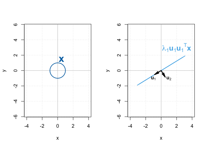
All vectors in $\mathbb{X}$ are transformed by ${\mathbf{A}}_1$, namely, stretched along ${\mathbf{u}}_1$ and shrunk to zero along ${\mathbf{u}}_2$. As a result, the initial circle became a straight line.

Previously, matrix $\mathbf{A}$ transformed vectors in $\mathbb{X}$ into an ellipse, another 2-D shape. And yet, matrix ${\mathbf{A}}_1$ transformed vectors in $\mathbb{X}$ into a line, a 1-D shape. Both $\mathbf{A}$ and ${\mathbf{A}}_1$ are symmetric. How come one preserves whereas the other reduces the dimension? In the next post, we will discuss the reason by introducing the concept of rank.